Week 4 - CHT Analysis on Exhaust port

 CONJUGATE HEAT TRANSFER (CHT) ON EXHAUST PORT

AIM 

To perform CHT analysis using Ansys Fluent.

GIVEN

exhaust port (Soliworks Part Document)

Inlet Velocity = 5m/s

Inlet Temperature = 700K

Outer Wall Convection = 20 W/m^2 K

Outlet Temperature = 300K

INTRODUCTION

The Conjugate Heat Transfer (CHT) analysis type allows for the simulation of heat transfer between solid and fluid domains by exchanging thermal energy at the interfaces between them. Typical applications of this analysis type exist as, but are not limited to, the simulation of heat exchangers, cooling of electronic equipment, and general-purpose cooling and heating systems.

Fig 1: Natural convection around a heat exchanger. Cold water enters in and gets heated due to hot air flowing opposite to it.

The CHT approach has an advantage over FE thermal analyses in that wall heat transfer coefficients and their local variations on surfaces are directly calculated within the model rather than based on simplified empirical calculations. The CHT approach therefore has benefits for those applications where heat transfer is either non-uniform or difficult to calculate empirically.

STEPS USED FOR SIMULATIONS

 

Click on red encircled "Workbench 2021 R2" as shown in the above image to start the simulation.

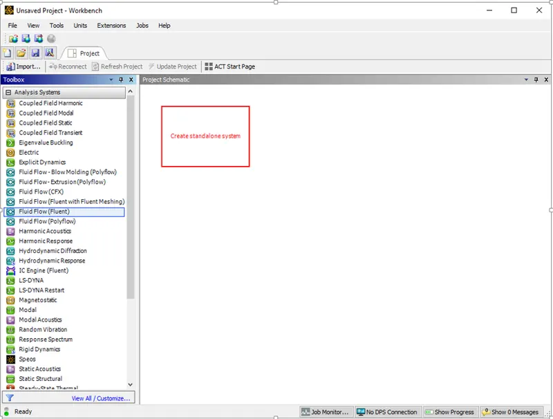
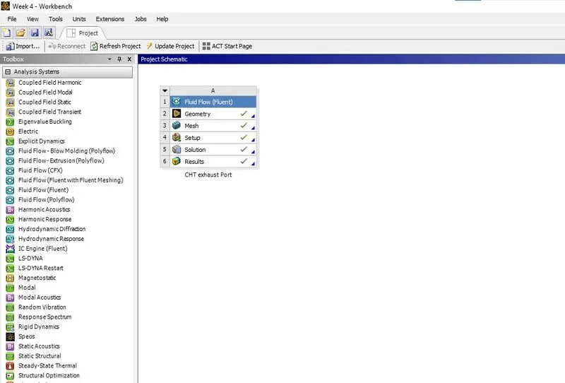
Click On Fluid Flow (Fluent) under Analysis Systems and drag it to create a standalone system.

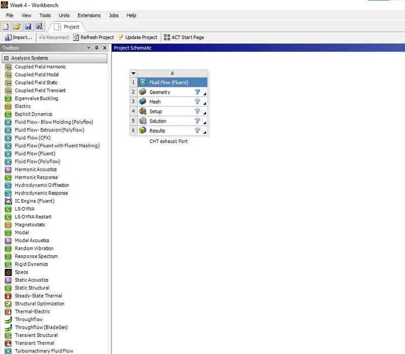
 Rename the Project by using the left click and then click the Geometry.

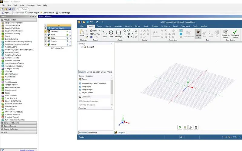
 On clicking the geometry, the Space Claim window opens as shown in the above image.

 

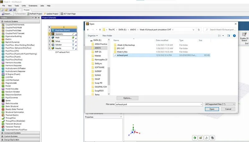
 Open the dowloaded exhaust port.STEP file as shown in the above image.

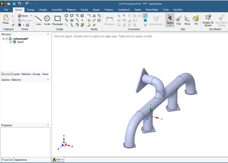
 The above image represents the screen after opening the step file in Space Claim.

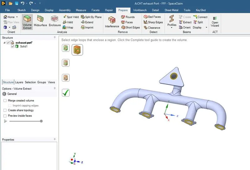
 Now we extract the fluid domain using volume extract and then selecting the edges as shown in the above image.

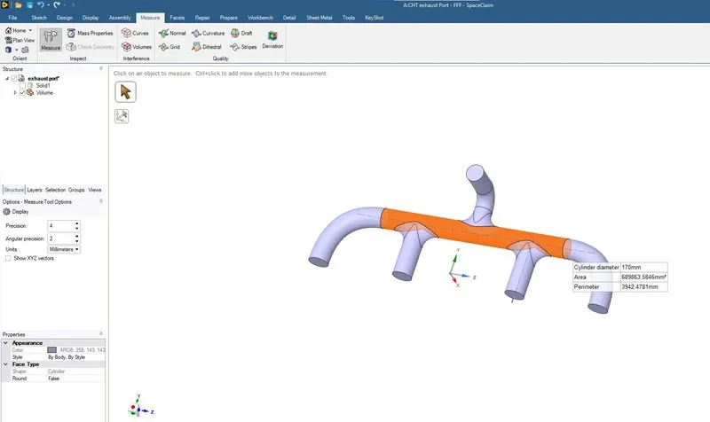
 The above image is the extracted fluid domain. by using the measure tool we get the parmeters required for setup.

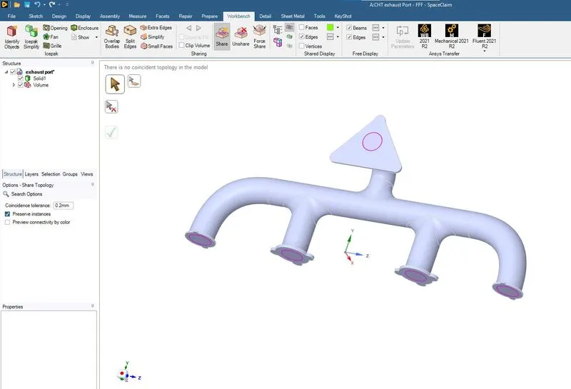
 We perform the the share topoloy using the Share under Workbench

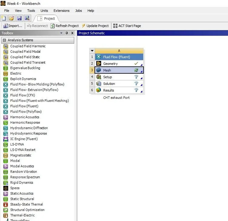
 The meshing module is started by clicking the Mesh in the workbench.

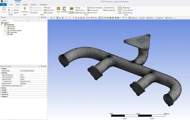
 By clicking the Generate Mesh the basic mesh is generated.

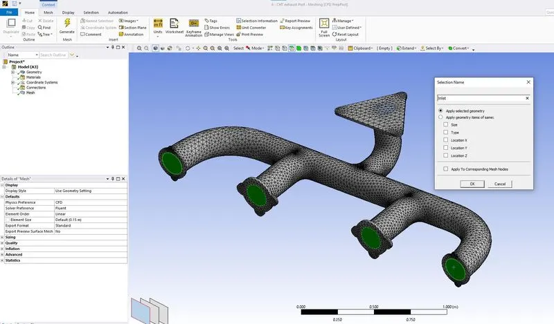
Using Named Selection the selected faces are named as Inlet.

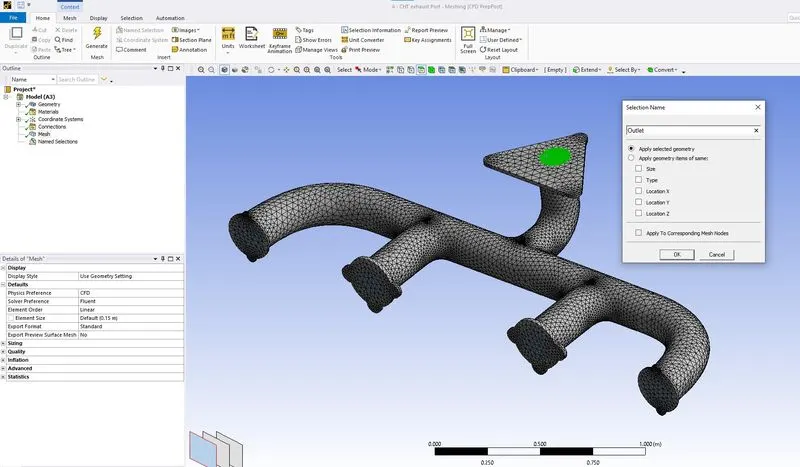
Using Named Selection the selected faces are named as Outlet.

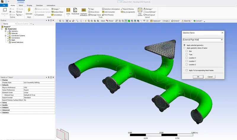
Using Named Selection the selected faces are named as External Pipe Wall.

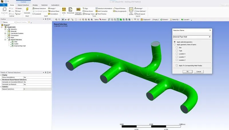
Using Named Selection the selected faces are named as Internal Pipe Wall.

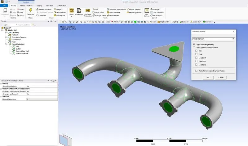
Using Named Selection the selected body is named as Fluid Domain.

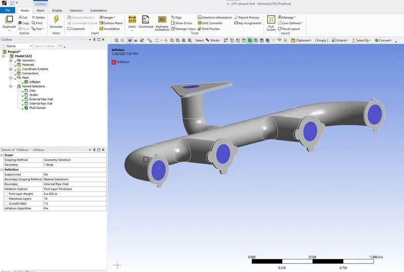
Using the inflation we define the inflation layer to be generated for the selected body as shown in the above image.

Using the online Y+ calculator we get the first layer thickness. the trailing images shown the values of first layer thickness estimated and boudary layer thickness.

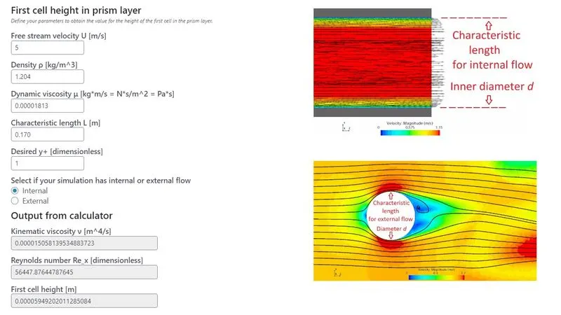
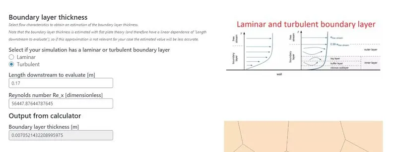
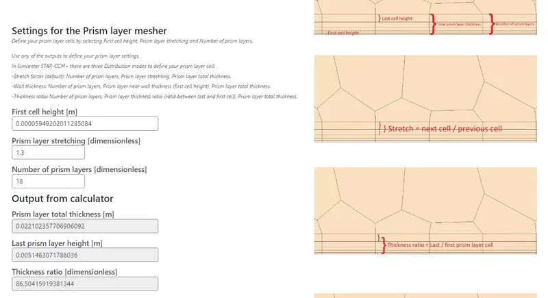
 Based on trial and error method we arrive at grwoth rate to 1.3 and Maximum nuber of layers to 18.

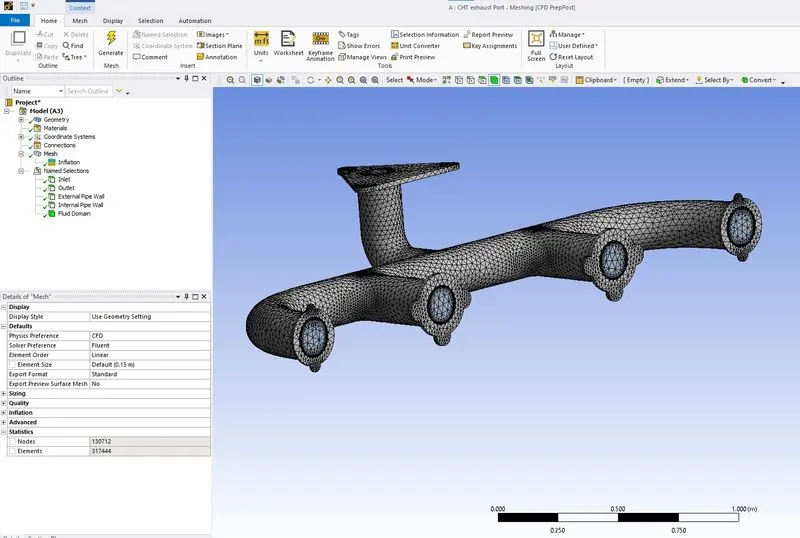
 Final Mesh elements are as shown in the above image.

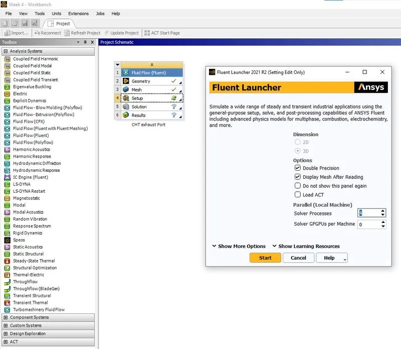
 Fluent Set up is started as shown in the above image.

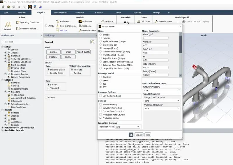
Energy is enabled in Physics tab since this is a thermal analysis. Viscous model selected is k-w SST as shown in the above image.

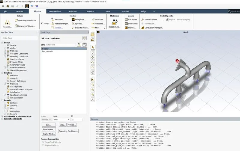
In the cell zone condition we set the type as solid for solid domain.

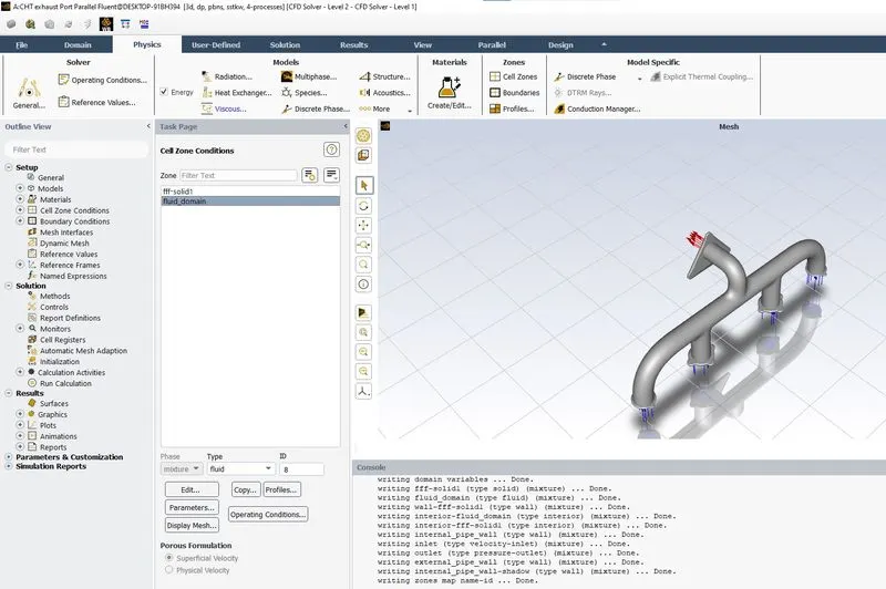
In the cell zone condition we set the type as fluid for fluid domain.

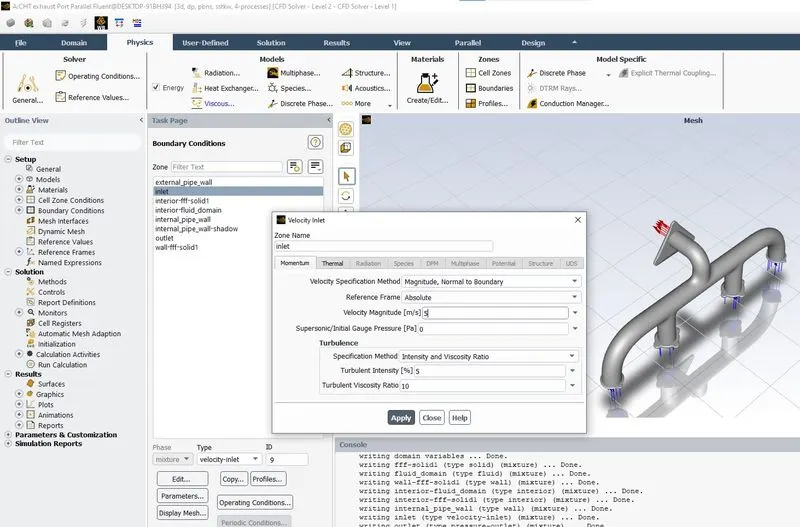
 Using the Boundaries under Zones in Physics tab the inlet velocity is set to 5m/s

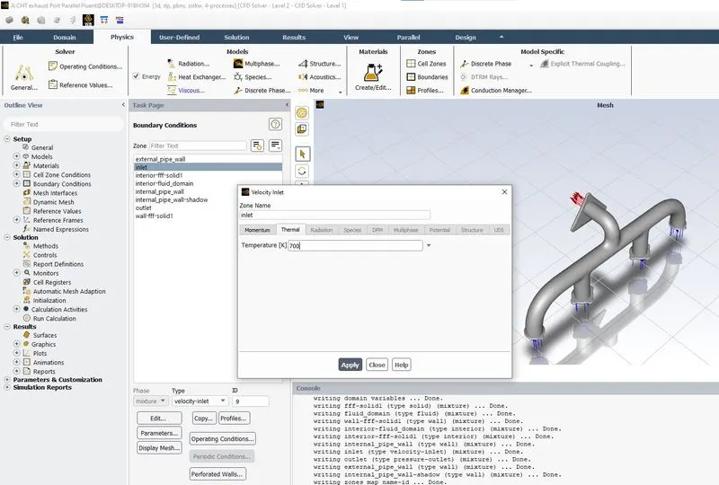
Using the Boundaries under Zones in Physics tab the inlet temperature is set to 700K as shown in the above image.

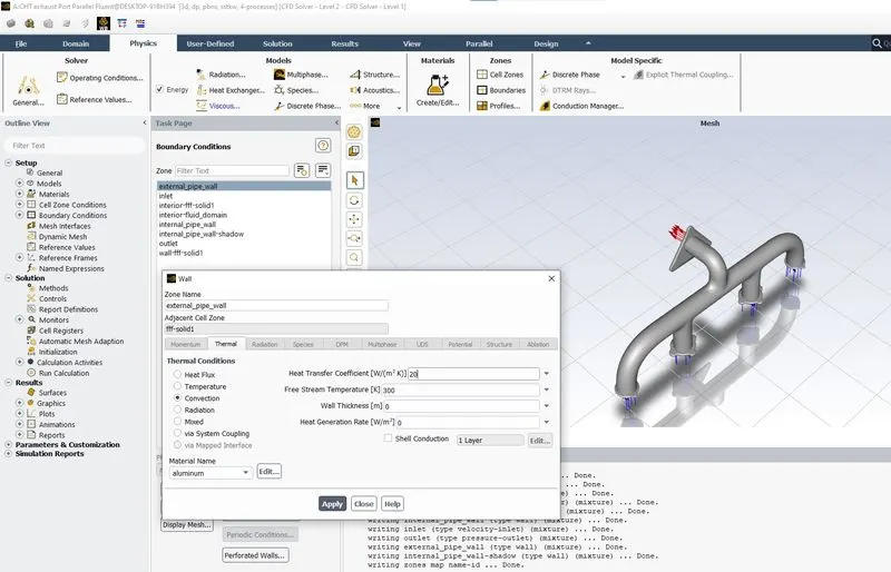
 Wall Boudary conditions are set as shown in the above image.

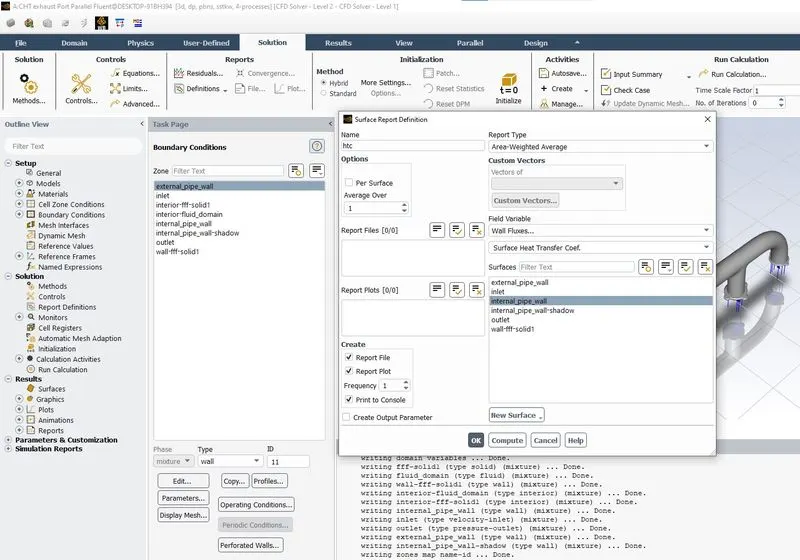
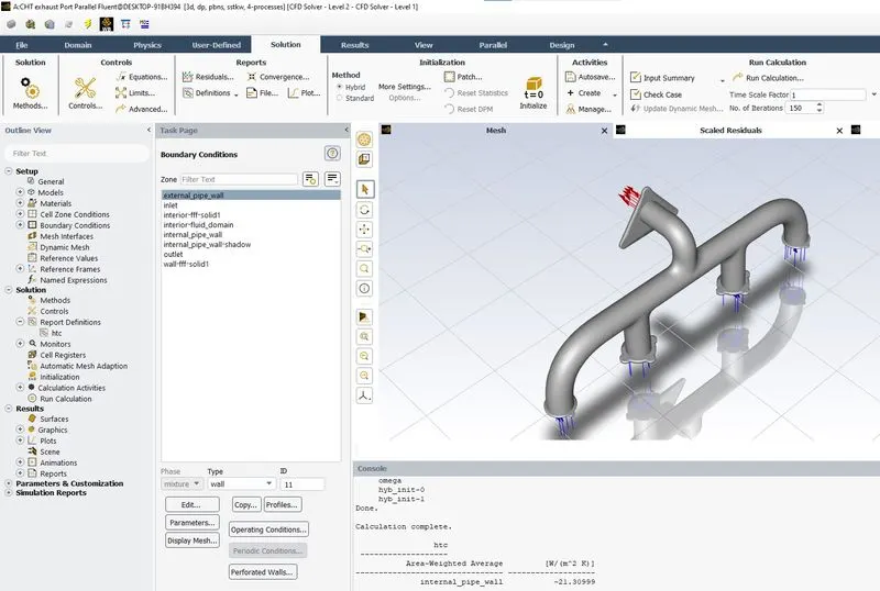
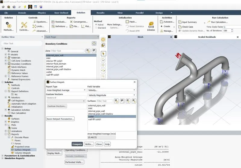
 Surface report is defined for surface heat transfer coefficient as shown in the above image.

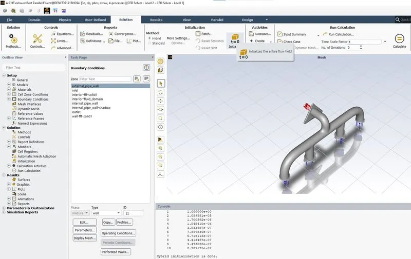
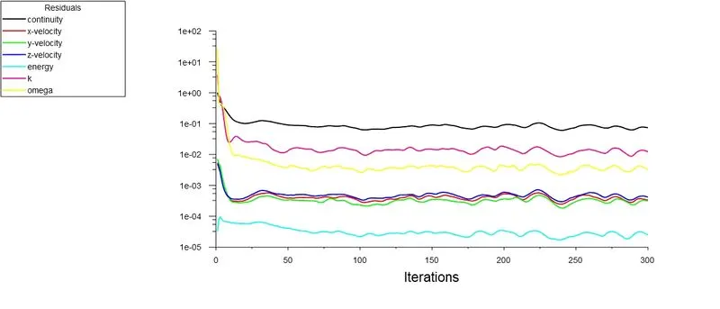
 Hybrid initialization is done and calculation is run for 300 iterations.

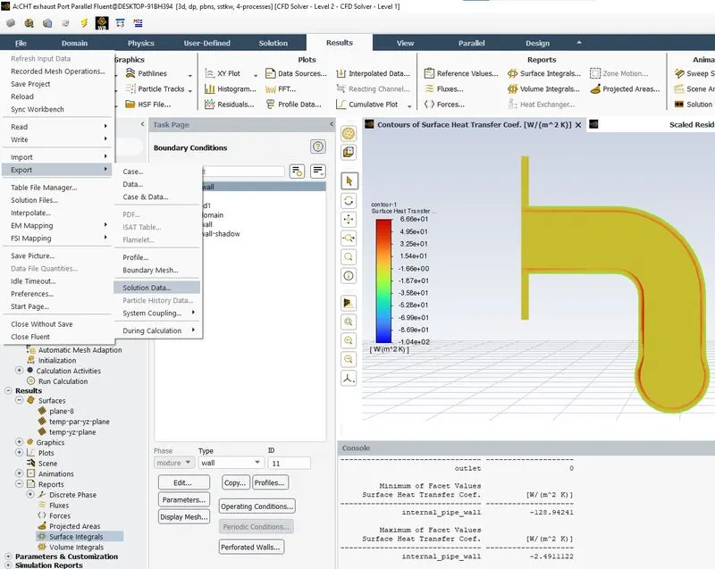
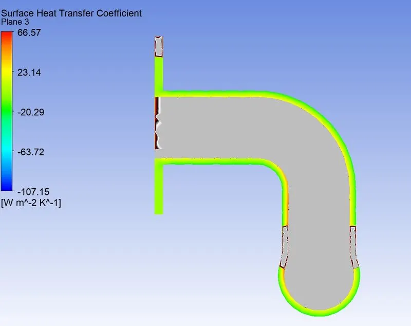
 The solution data is exported so that we can load the results in CFD post for vieiwing the surface heat transfer coefficient.

Case done using ANSYS Fluent

 1.1 Scaled Residuals

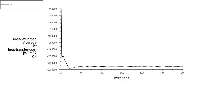
 1.2 HTC (Heat Transfer Coefficient) Plot

 1.3 Computation of Heat Transfer Coefficient

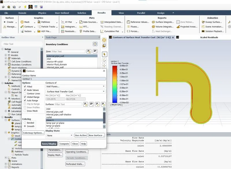
 1.4 Contours of Surface Heat Transfer Coefficient

 1.5 Computation of Maximum Surface Heat transfer Coefficient

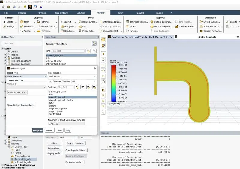
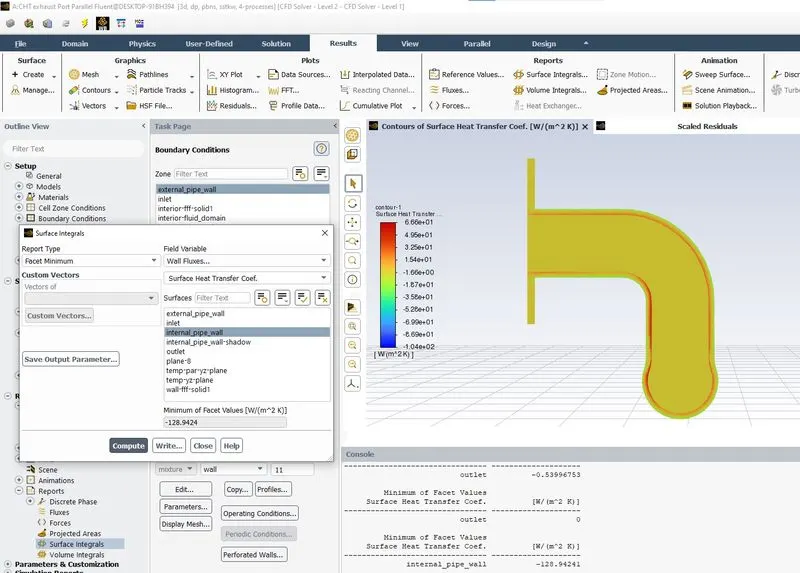
 1.5 Computation of Minimum Surface Heat transfer Coefficient

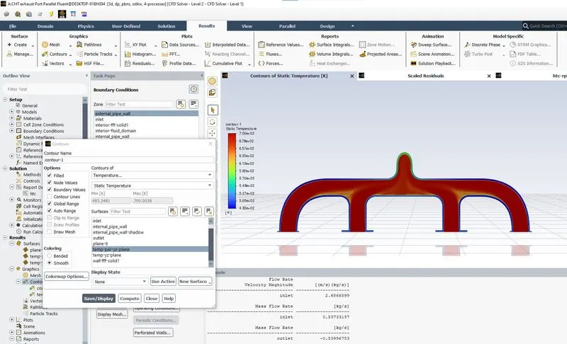
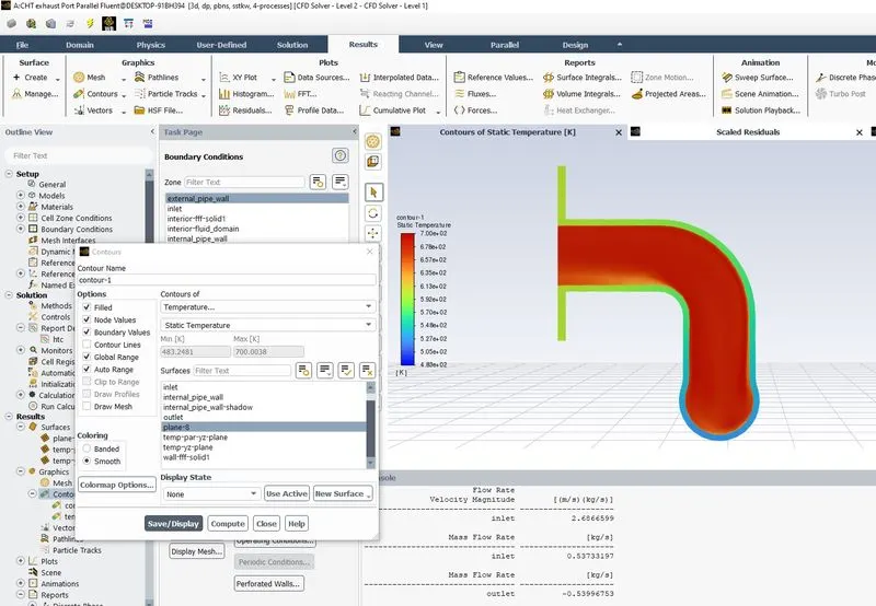
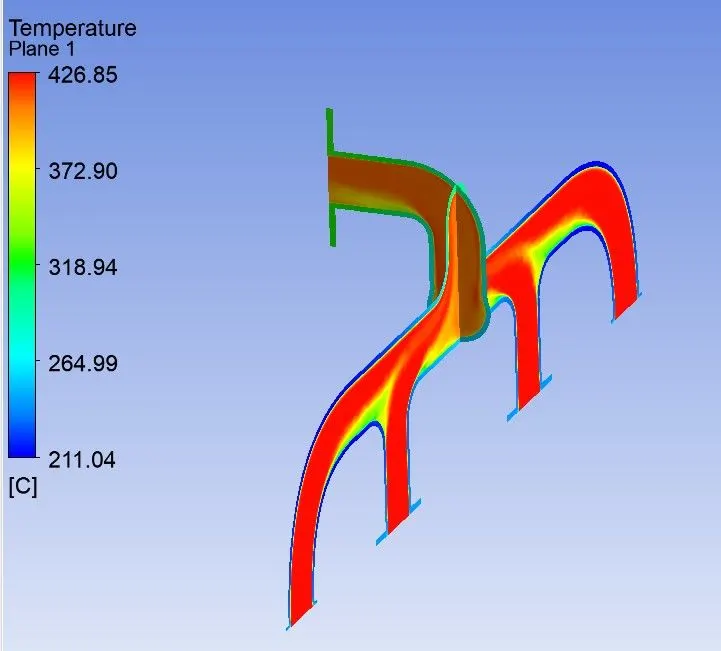
 1.6 Temperature Contour in XY Plane

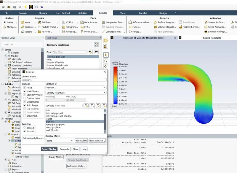
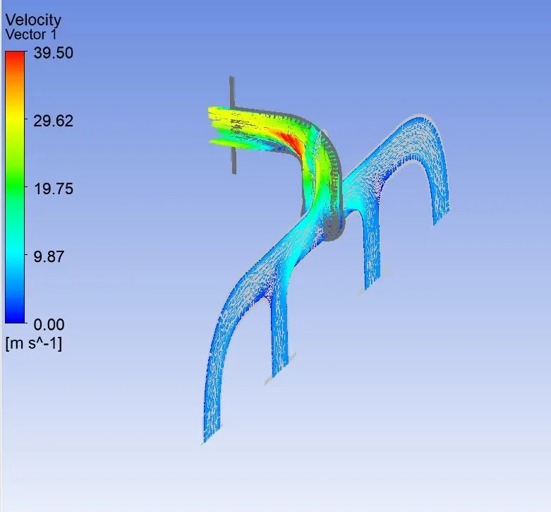
 1.7 Velocity Contour in XY Plane

  

 

 

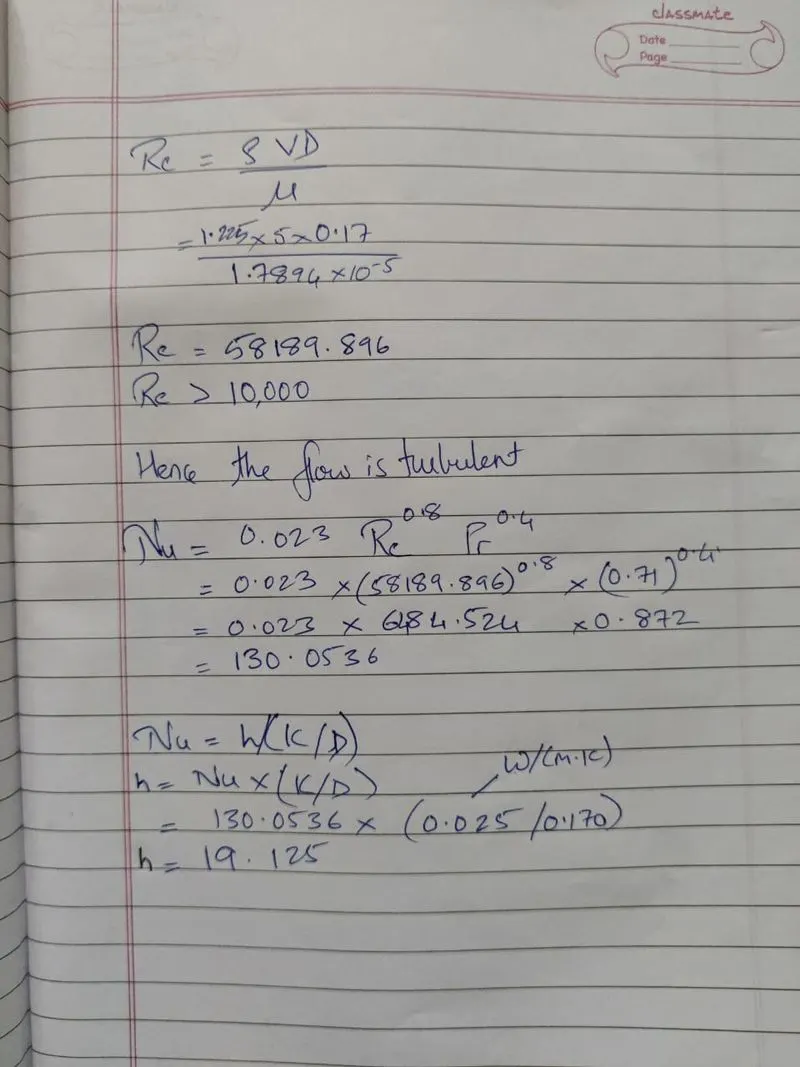
1.8 Manual Calcuation of Heat TranSfer Coefficient

Nusselt Number (Nu)

The Nusselt number is the ratio of convective to conductive heat transfer across a boundary. The convection and conduction heat flows are parallel to each other and to the surface normal of the boundary surface, and are all perpendicular to the mean fluid flow in the simple case.

where

h is the convective heat transfer coefficient of the flow

L is the characteristic length

k is the thermal conductivity of the fluid

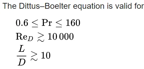
The Dittus–Boelter equation (for turbulent flow) as introduced by W.H. McAdams is an explicit function for calculating the Nusselt number. It is easy to solve but is less accurate when there is a large temperature difference across the fluid. It is tailored to smooth tubes, so use for rough tubes (most commercial applications) is cautioned. The Dittus–Boelter equation is:

SUMMARY

Using Ansys Fluent, the Heat transfer Coefficient computed is -21.30999 W/m^2 K

Analytically the Heat Transfer Coefficient calculated is 19.125 W/m^2 K

CONCLUSION

Conjugate heat transfer analysis is done for exhaust port using Ansys Fluent.

Y+ value has been acoording to the turbulence model selected

The wall/surface heat transfer coefficient on the internal solid surface has been calculated and verified analytically.

The velocity & temperature contours in appropriate areas has been plotted.