Week 4 - CHT Analysis on Exhaust port

Aim: Perform a CHT analysis on an export port of an automobile.

Theory:

The Conjugate Heat Transfer (CHT) analysis type allows for the simulation of heat transfer between solid and fluid domains by exchanging thermal energy at the interfaces between them. The conduction mode of heat transfer being a dominant mode of heat transfer in solids oftenly while convection being the dominant mode of heat tansfer in fluids oftenly. Typical applications of this analysis type exist as, but are not limited to, the simulation of heat exchangers, cooling of electronic equipment, and general-purpose cooling and heating systems.

The exhaust port of an automobile is one such application of CHT analysis where the hot burnt gases flow out of the cylinders into these port which combine into a common exhaust to form an exhaust manifold. The manifold carry these hot gases further down the exhaust system which release these gases to atmosphere while the whole system conducting and convecting the heat to the atmosphere through their boundaries themselves.

Setup:

1. Setting up the geometry
   Set up fluent case in Project schematic and import the geometry in space claim.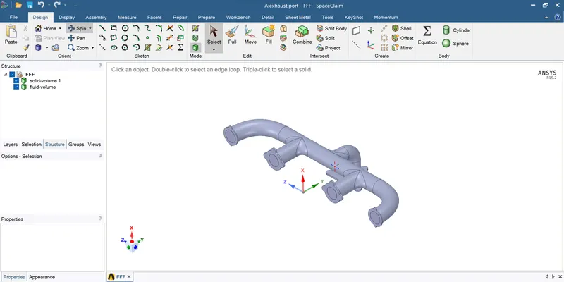
   
   
   
   The inside volume of the geometry is extracted to form the fluid domain for the hot exhaust gas flow.
   
   
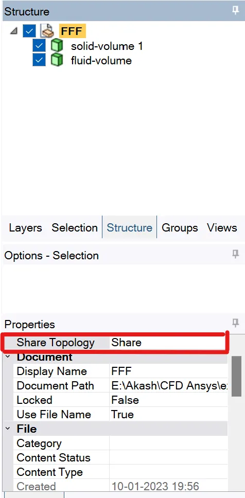
   The extracted volume and the solid body is moved together under same component (FFF). For continous flow of information across the solid-fluid interface the topological properties are shared. This shared topology property is communicated to further processes like meshing and solver using 'share' option under workbench ribbon.
   
   
   
   
2. Meshing
   Inflation at solid-fluid interface is provided. Also, body sizing control is used to further refined the default generated mesh.
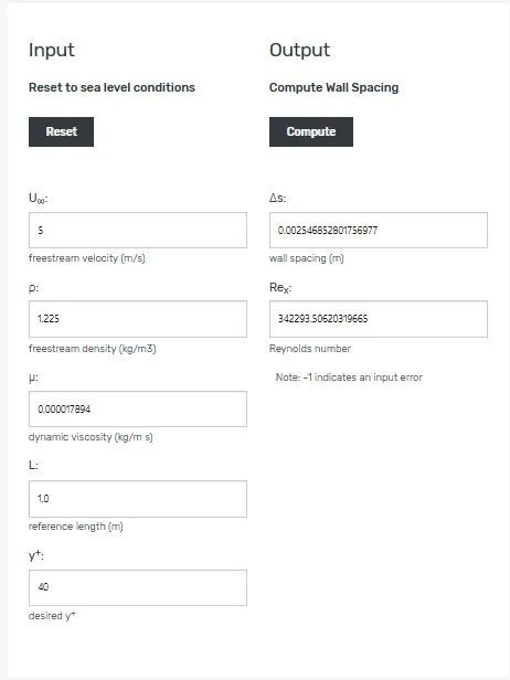
   Total inflation layer thickness option was chosen for inflation layers. The first layer thickness was calculated based on y+ value of 40, which is suitable for high reynolds number flow.
   
   
   
   
   
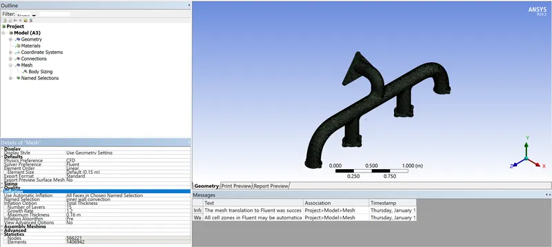
   Quality of mesh was also found to be satisfactory.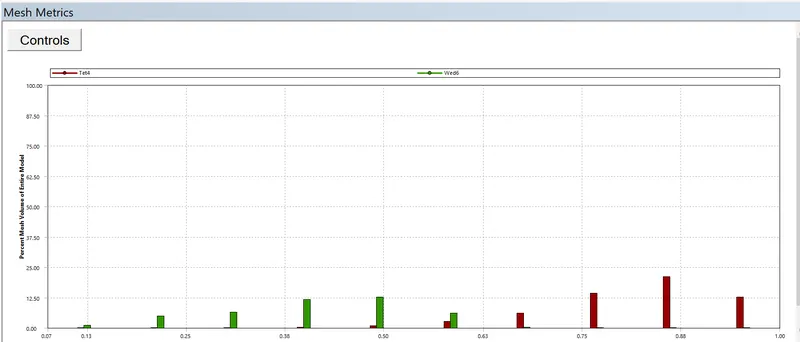
   
   
   
   Aspect ratio was also satisfactory with majority of elements having aspect ratio closer to 1.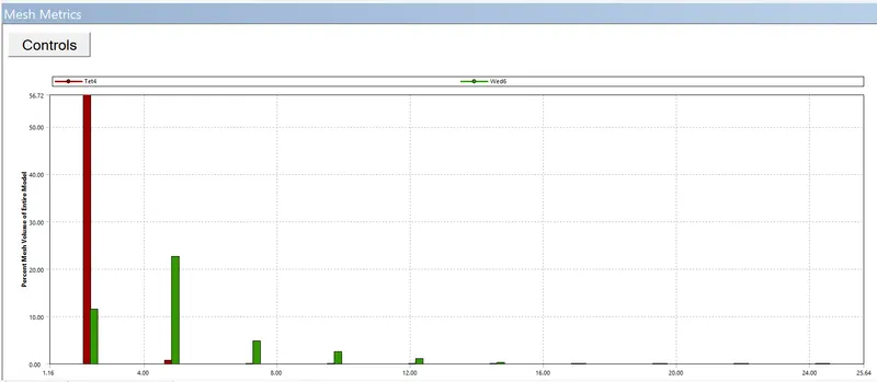
   
   
   
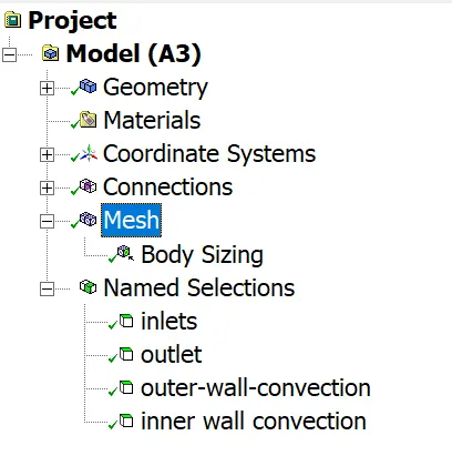
   Faces and Boundaries were named.
   
   
3. Solving
   Since y+ value of 40 was chosen, we must use a high reynolds flow solver like `k-epsi`turbulent viscous model. Also, as heat transfer is also involved we will use energy equation as well.
   The material for fluid is air and for solid it is aluminium.
   
   
   
   Boundary Conditions were provided.
   Inlet velocity = 5 m/s.
   Inlet temperature = 700 K.
   Hea transfer coefficient on outer convective surface = 20 W/`W/(m^2.K)`.
   Adiabatic wall condition on the rest of the surfaces.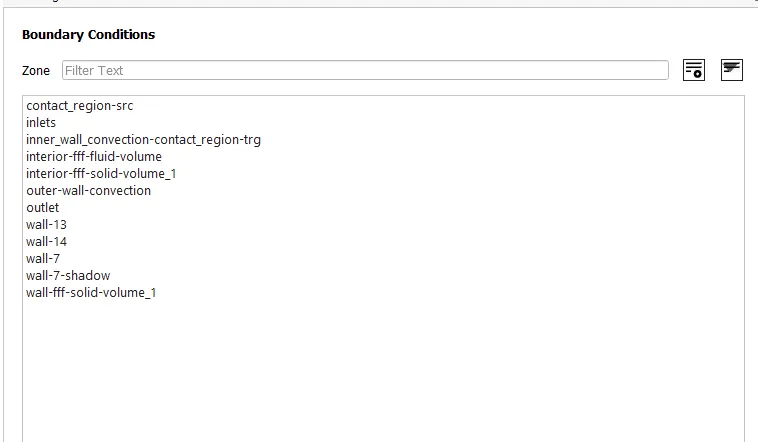
   
   
   
   
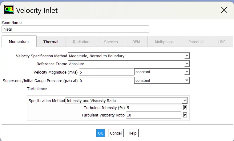
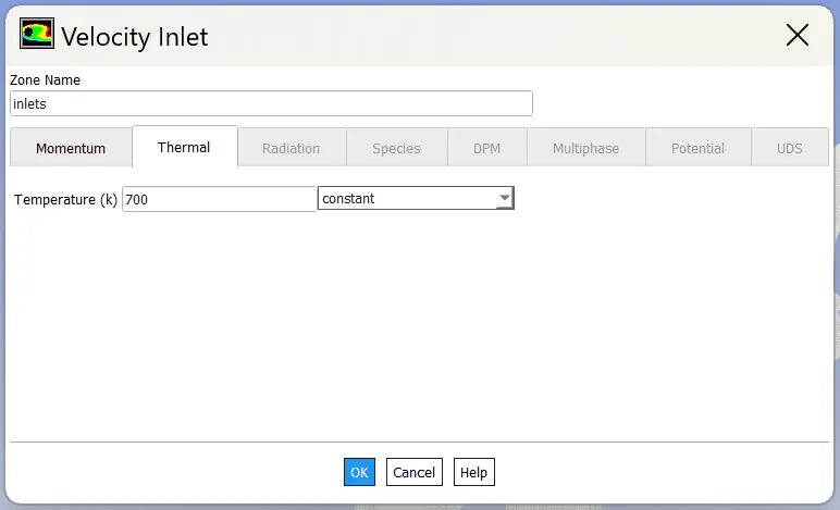
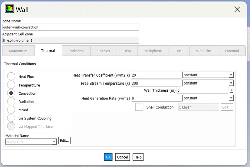
   Solution is initialized; contour plots and solution animations files are created.
   
   Finally the solution was made to run for 300 iterations. With each iteration contour plots and scaled residue plots are updated.
   
   
4. Results:
   
   Following plots were obtained after completion of given number of iterations.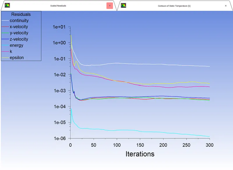
   
   
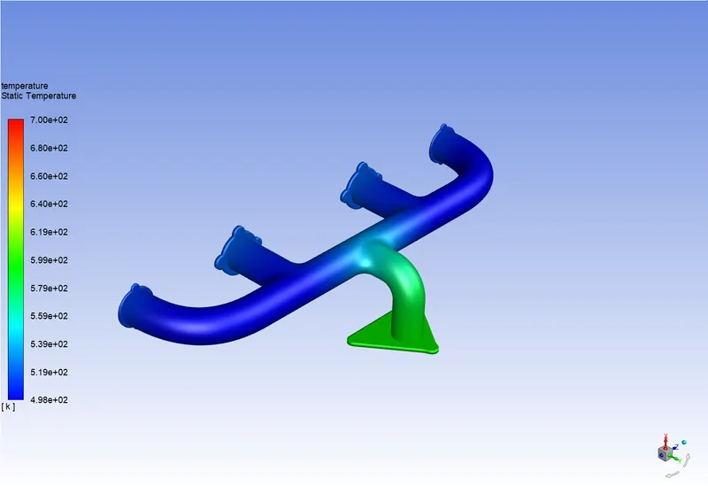
   scaled residue plot temperature contour plot
   
   For obtaining the heat transfer coefficient plot we have to export the solution data is .cdat format to view in result window of the case.
   
   exporting solution data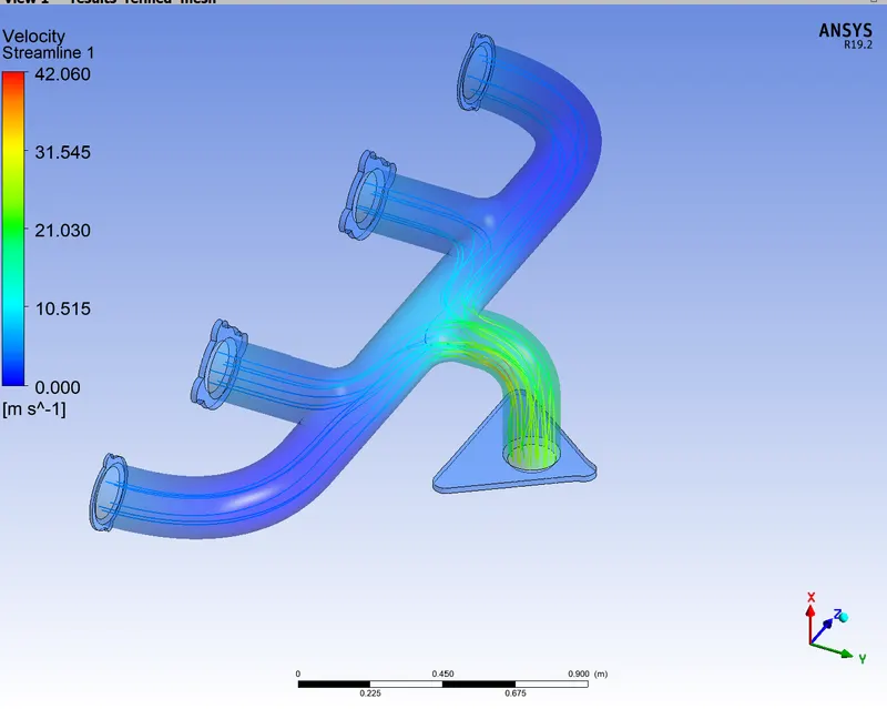
   
   streamline plot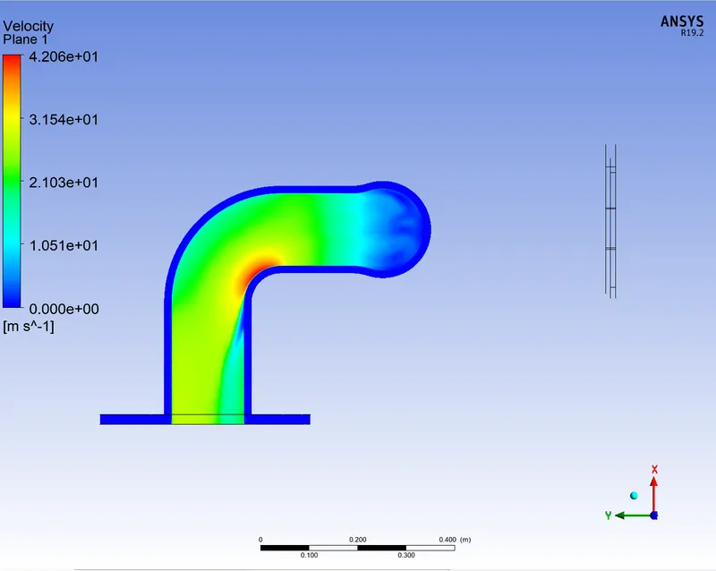
   
   
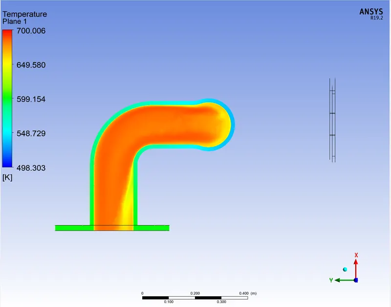
   velocity plot at outlet section temperature plot at outlet section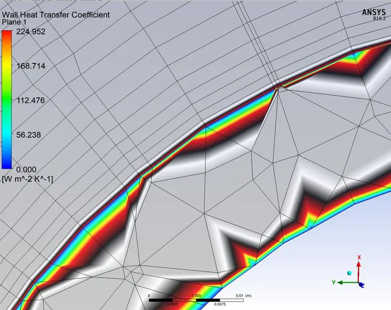
   
   
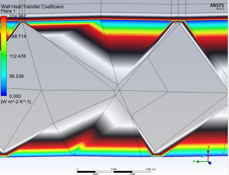
   high heat transfer coefficient coefficient region low heat transfer coefficient coefficient region
   
   From above plots, it is seen the inner bend region in outlet section the fluid has the highest velocity (around 42 m/s).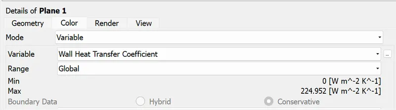
   
   
   Maximum heat transfer occurs in maximum velocity region and its value is 224.952 `W/(m^2.K)`.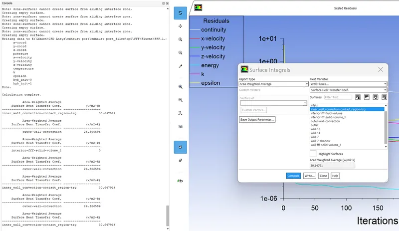
   
   
   
   We ran the same case with k-omega SST model. Few modifications required were, changing y+ value to <5 and geometry mesh. For y+=3 first layer first layer thickness came out to be 0.00019 m.
   
   
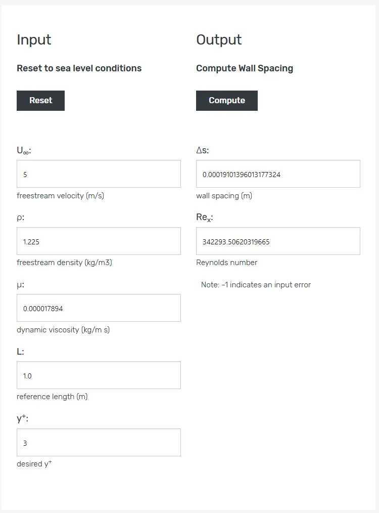
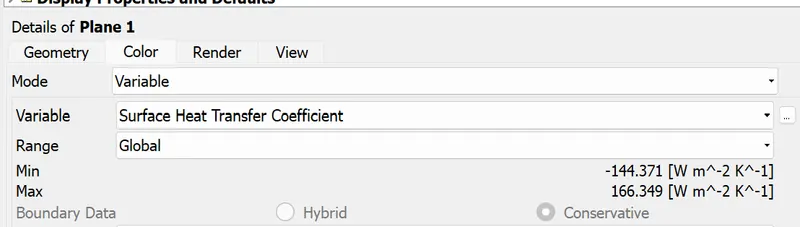
   first inflation layer thickneess max heat transfer coefficient (k-omega SST)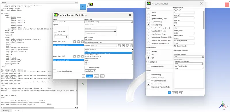
   
   
   area weighted average heat transfer coefficient
   
   Verifying the results:
   
   Using Colburn relation `Nu=0.023Re^0.8Pr^(1/3)`
   k of air at bulk mean temperature of 500K=0.0407 `W/(m.K)`
   `Pr=(mu.c_p)/k =0.6815 `
   `Re=(rho.v.D)/mu=56833.42` where D is 0.165m
   `Nu=111.39=(h.D)/k`
   `h=27.479``W/(m^2.K)`
   
   The results we got for `k-epsi`model : weighted average heat transfer coefficient = 30.64`W/(m^2.K)`which leads to error of 11.5%.
   
   The results we got for `k-omega`SST model: weighted average heat transfer coefficient = 27.89 `W/(m^2.K)` which leads to error of 1.4%
   
   However, exhaust ports are generally made from 'Ductile-Cast Iron' or 'Stainless Steel SS304' (with k-epislon for reduced computation time).
   
   For Ductile-Cast Iron following results were obtained: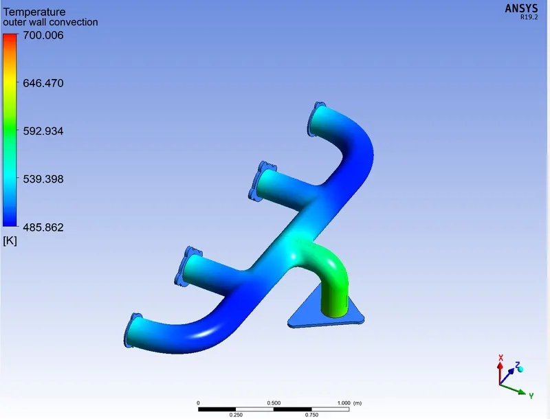
   
   
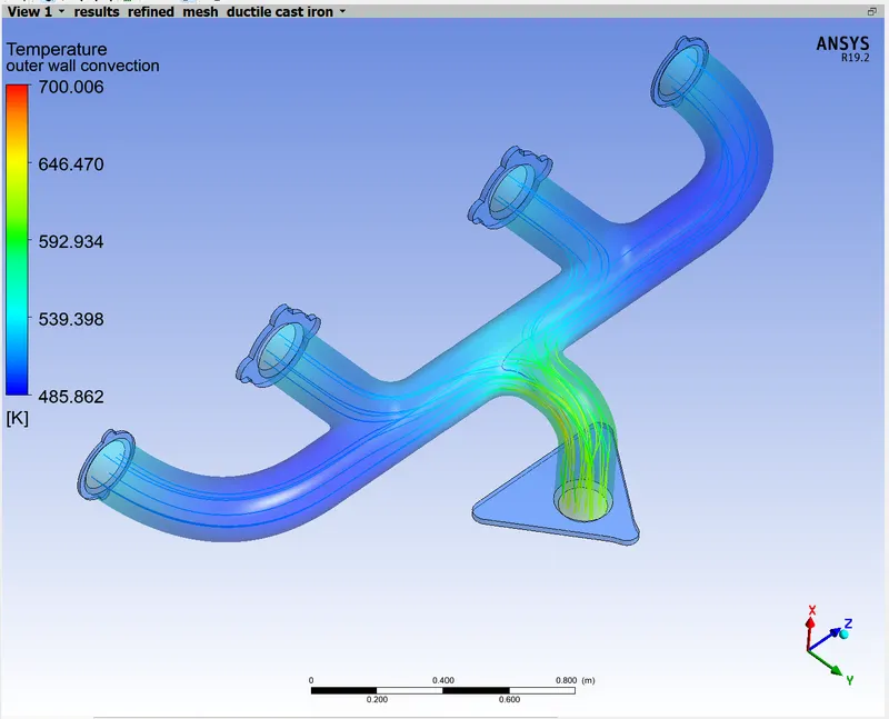
   temperature contour plot streamline plot
   
   
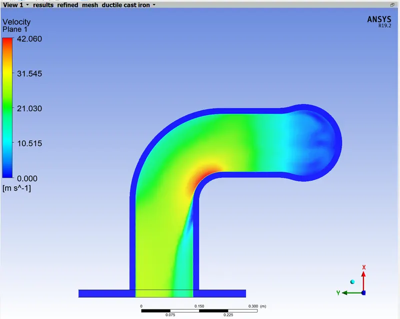
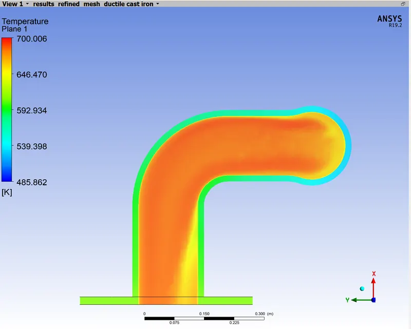
   velocity at outlet section (Ductile-Cast Iron) temperature at outlet section (Ductile-Cast Iron)
   
   The same region as in case of aluminum has maximum velocity and highest heat transfer coefficent value (751.675 `W/(m^2.K)`). But comparitively, ductile cast iron has a higher maximum heat transfer coefficent value.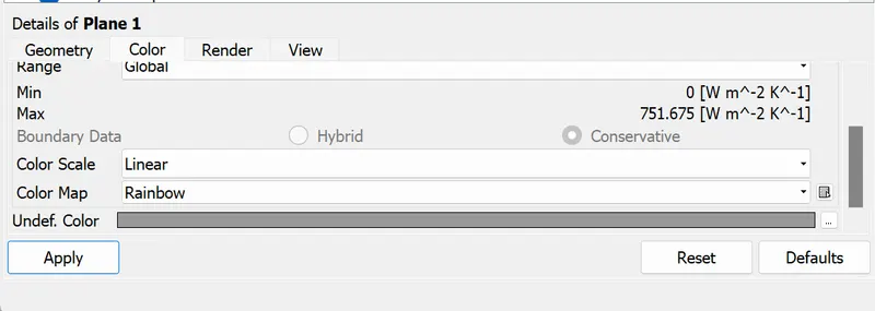
   
   
   
   For Stainless Steel SS304 following results were obtained: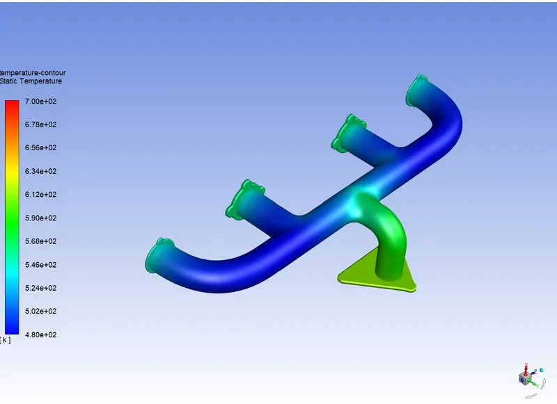
   
   
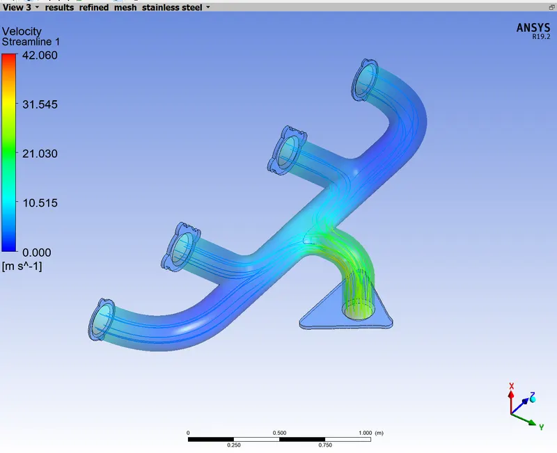
   temperature contour plot streamline plot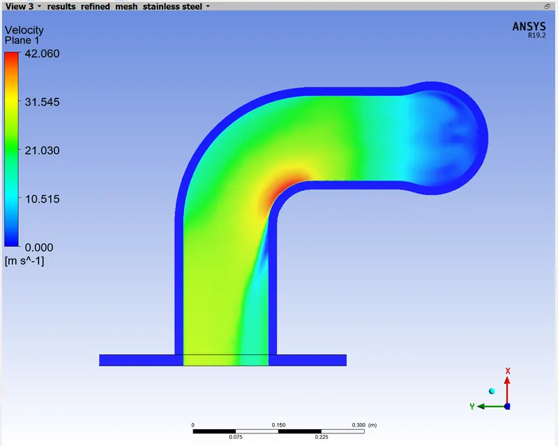
   
   
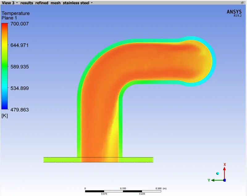
   velocity at outlet section (Stainless-Steel) temperature at outlet section (Stainless-Steel)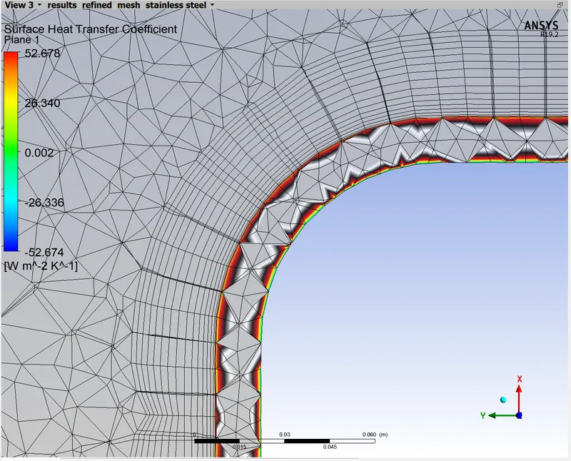
   
   
   maximum heat transfer coefficient (Stainless-Steel)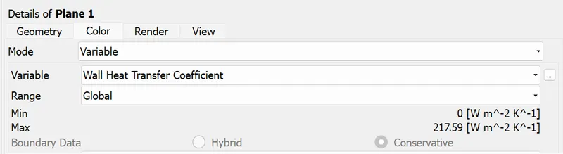
   
   
   The Maximum heat transfer coefficient came out to be 217.59 `W/(m^2.K)`.
   
   Above cases highlighted the variation in simulation results based on material selection for exhaut port. We shall study the effect of variation in flow paramters on simulation results.
   
   Flow Velocity 25 m/s: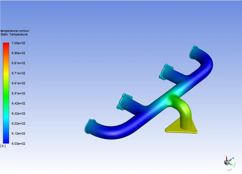
   
   
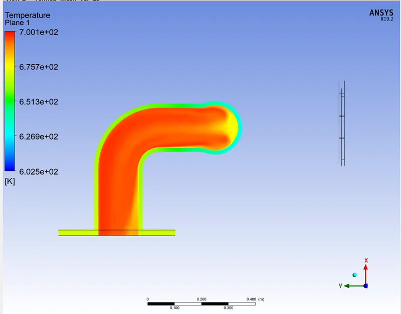
   temperature contour plot (vel 25 m/s) temperature at outlet section (vel 25 m/s)
   
   
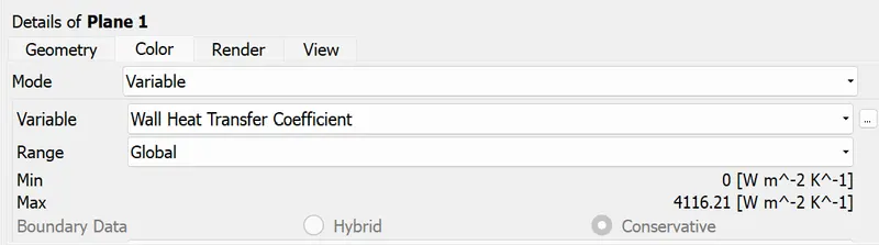
   maximum heat transfer coefficient (vel 25 m/s)
   
   
5. Conclusion:
   
   Following inferences can be made from the simulation above-
   

• The flow mixing at the common outlet enterance and larger junction area leads to lower velocity giving ample time for solid to conduct heat from inner surface to outer surface. This leads to maximum temperature around the region.
• Since mass flow rate is same, also outlet having smaller area than inlets leads to increase in outlet velocity and hence the higher Reynold Number of the flow. A higher Reynold Number implies higher heat transfer coefficient which is consistent with out velocity and heat transfer coefficient plot.
  As Nu`prop`Re for convection and `Nu=(h.L_c)/k also `Re=(rho.v.L_c)/mu` where, Nu is Nusselt number, Re is Reynolds number, `L_c`is characteristic length, `mu` is dynamic viscosity, `rho` is density of the fluid and k is thermal conductivity of the solid .
  Therefore, `hpropv`.
• Increasing velocity will increase the overall wall heat transfer coefficient as evident from the plots. The high velocity case (25 m/s) has much more uniformly distributed temperature profile than the lower velocity flow case (5 m/s).
• The k-omega SST model gave better results for weighted average heat transfer cofficient at the wall compared to k-epsilon model. The reason is that as heat transfer coefficient is calculated aat the wall, the k-omega model is better for capturing near wall phenomena while k-epsilon works better for capturing flow phenomena away from the wall.