Week 4 - CHT Analysis on Exhaust port

AIM

To perform the steady-state conjugate heat transfer simulation on the exhaust port when the air is coming at the inlet at a speed of 5m/sec.

Objective:

1. Give a brief description of why and where a CHT analysis is used.
2. Maintain the y+ value according to the turbulence model and justify the results. 
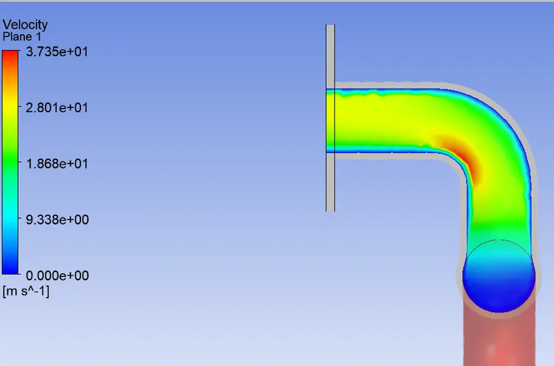
3. Calculate the wall/surface heat transfer coefficient on the internal solid surface & show the velocity & temperature contours in appropriate areas.
4. How would you verify if the HTC predictions from the simulations are right? On what factors does the accuracy of the prediction depend on?

1.Conjugate Heat Transfer anlysis:

 Conjugate heat transfer analysis is based on the mathematical structure problem which describes the heat transfer between the body and the fluid flowing over or inside it as a result of interaction between two objects. At the matching interface, the details are provided for temperature distribution and heat flux along the interface eliminating the need of calculating the heat transfer coefficient.

CHT analysis type allows for the simulation of the heat transfer between the solid and liquid domains by exchanging thermal energy at the interface between them. The simulation of the heat exchangers, cooling of the electronic equipment, and general-purpose cooling and heating system.  In the case of CHT that is being done in this project, we have the convection mode of heat transfer between the fluid and the solid aluminum wall of the exhaust pipe and then the conduction mode of heat transfer is followed within the wall of the exhaust pipe wall.

Solving and modelling approach:

1) The exhaust pipe was modeled in the space claim.

2) The exhaust port is a three dimensional model containing four inlets and one outlet. Despite having the isothermal boundary condition and a uniform flow rate at the four inlets the model can not be cut into two halves to save computational power. Therefore the whole model needs to be discretized it is also called as space discretization.

3) CHT analysis requires the both the solid and the liquid volume under consideration spaceclaim gives an option of volume extract for selecting the edges for fluid volume.

4) Both the solid component and the liquid component are copied into one component.

5) Share topology is created.

6) Spaceclaim gives an option for share coincident topology when share coincident topology is selected and executed. The , mesh from the fluid volume and the solid volume are said to be conformal with each other which is a requirement for the CHT analysis.

7) The exhaust port is loaded with the proper geometry and it is then si9mulated for the baseline computer generated mesh and in the next half we are going to be when we are going to use the refined mesh using the inflation layer and the element size is to be updated to required and hence a finer result is obtained.

8) The named selection is created like the inlet one, outlet one, and the outlet and the wall-convection is created to study thye effect of convection from the fluid to the wall and from the wall the heat is dissipated by the heat conduction method.

The geometry in the spaceclaim-

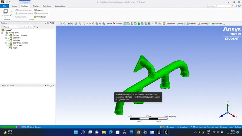
Inside the spaceclaim the extra edges were found in the geometry that was provided we have to removed by the option of prepare and the six edges were removed.

2) Then the volume extraction tool is used for the five edges and the volume and the process of fluid volume extraction is used for the edges to create the fluid volume.

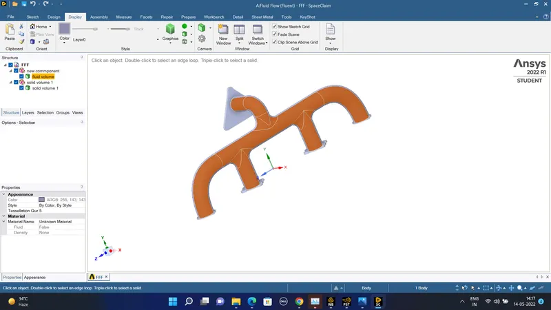
The solid volume is created -

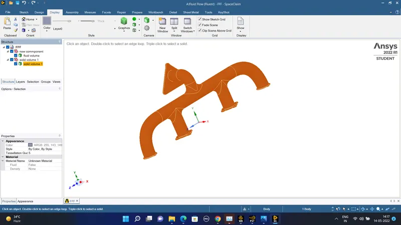
The solid and the fluid volume is created in the new component and it is kept inside it-

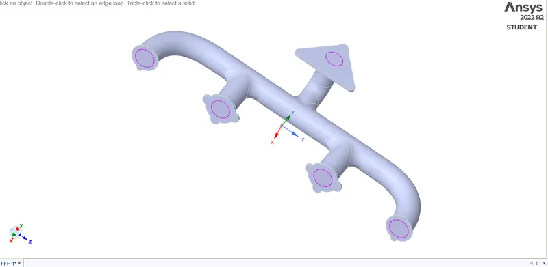
 BASE LINE MESH :

create named selection such as inlet; outlet; wall convection and inflation layer in between two volumes.

The baseline mesh that is created due to the original geometry with less modifications-

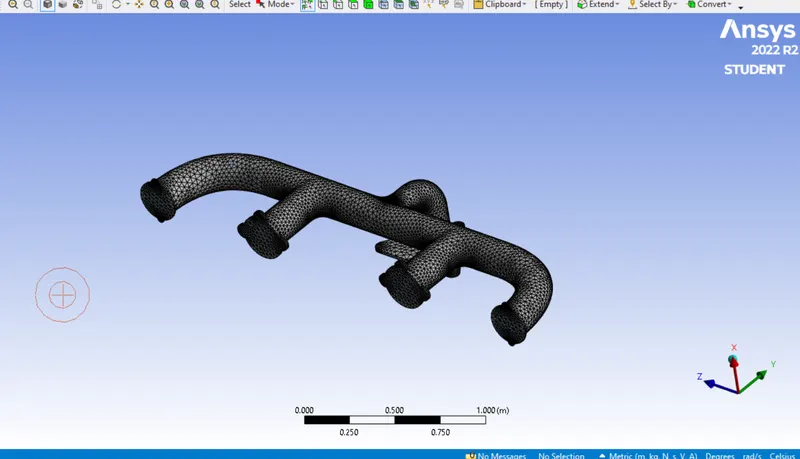
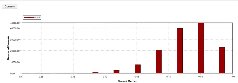
Mesh quality is that it conatins 138405 elements with default size of 150mm.

#) Then it is imported in the fluent solver to perform the CHT flow heat transfer analysis-

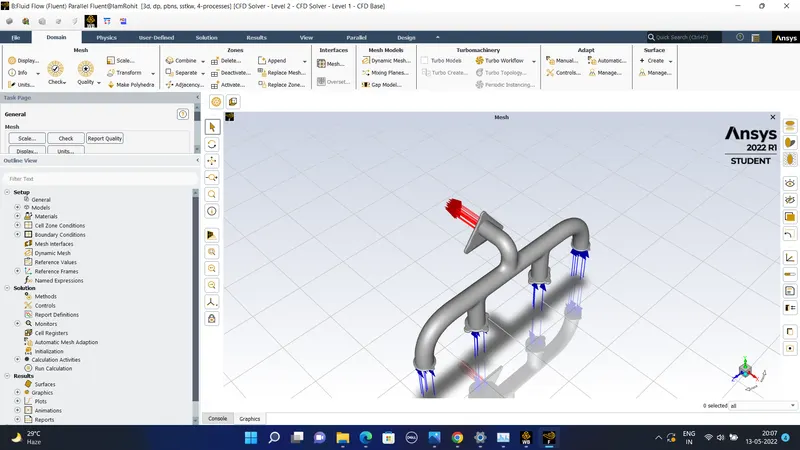
The following inputs of the varibale is made into the following velocity v = 5 m/sec at the inlet with the temperature of the fluid to be 700 kelvins. The boundary condition applied at the inlet is of  velocity inlet.

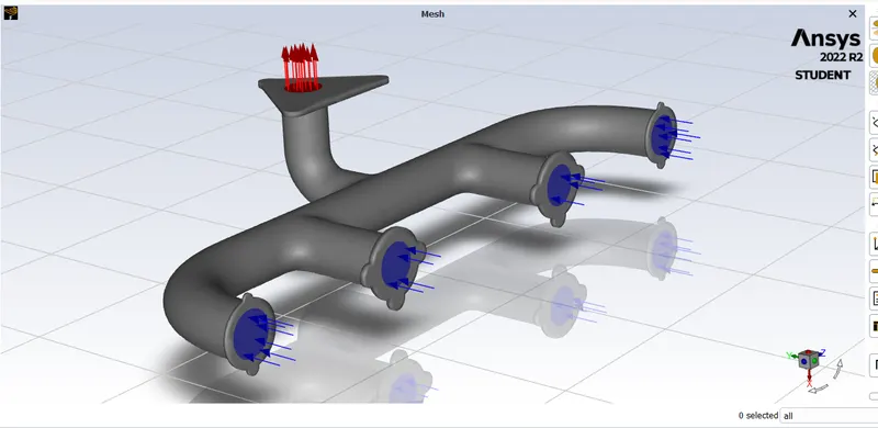
The red arrow indicates the outlet the boundary condition is of the pressure outlet type-

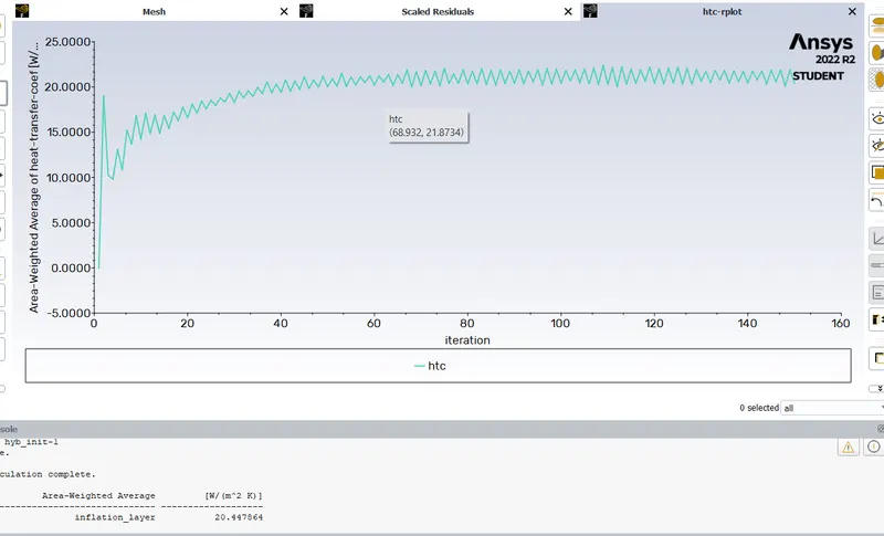
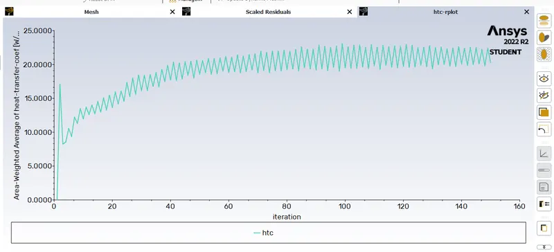
create defenition report on htc on inflated layer 

after initializing creatye contour for velocity and temperature

The third boundary condition is applied to the outer wall with a heat transfer coefficient of k = 20 w/m^2-k .

The steady state pressure based solver is used with the SIMPLE algorithm and the turbulence model that is used of the k- epsilon turbulence model is used with the outlet Gauge pressure = 0 pa and the energy equation is turned on.

material properties-

Fluid -

Fluid name = air.

Density = 1.225 kg/m^3

Specific heat = 1006.43 J/kg-k

thermal conductivity = 0.0242 w/m-k

viscosity = 1.789e-5 kg/m-sec.

Solid -

the solid material is of aluminum

Specific heat = 871 J/kg-k .

Thermal conductivity = 20 w/M-k

let us solve the model by three different solution methods such as

1. simple
2. simplec 
3. coupled

1.simple

2.simplec:

3.coupled:

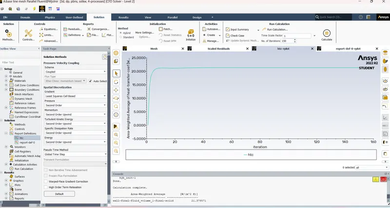
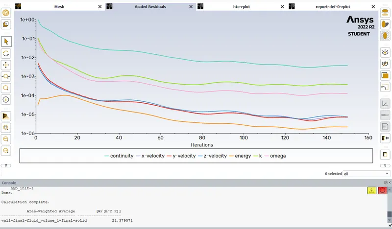
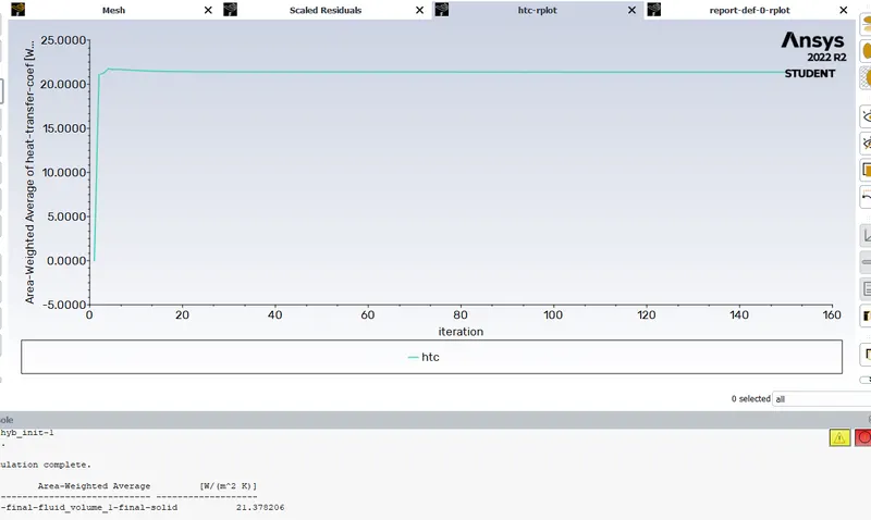
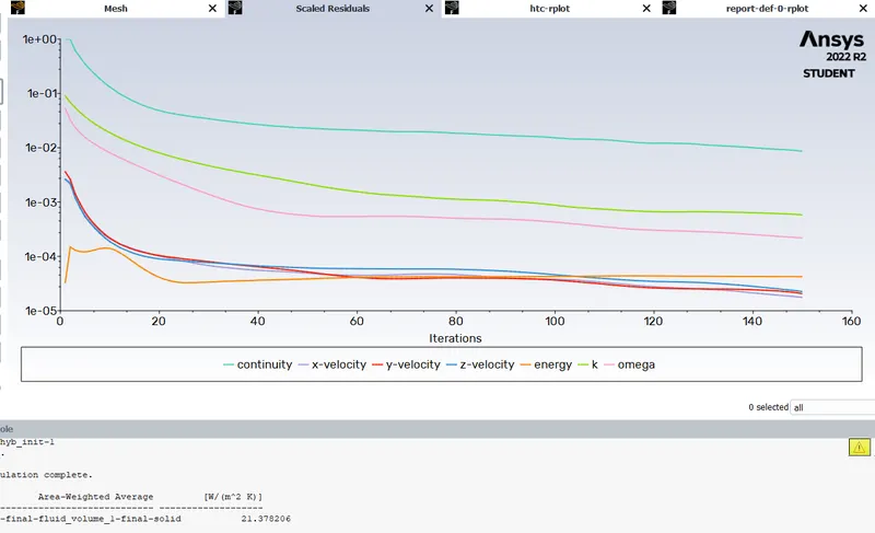
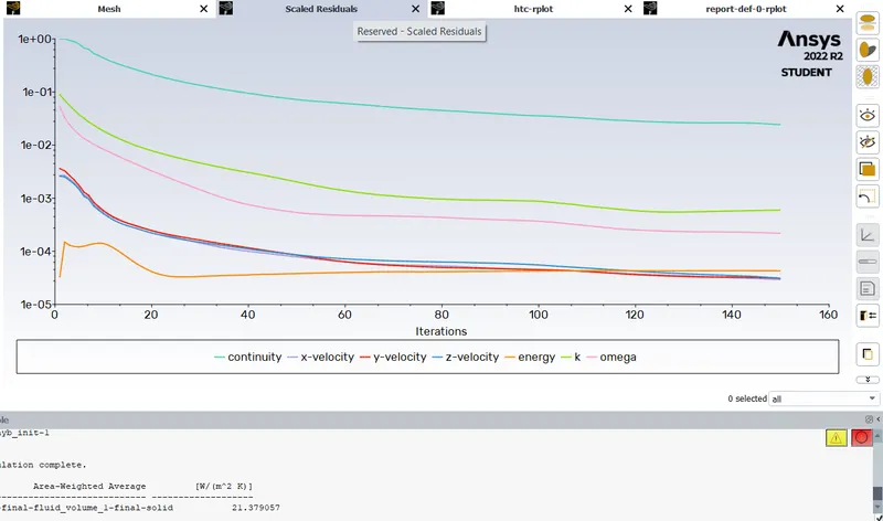
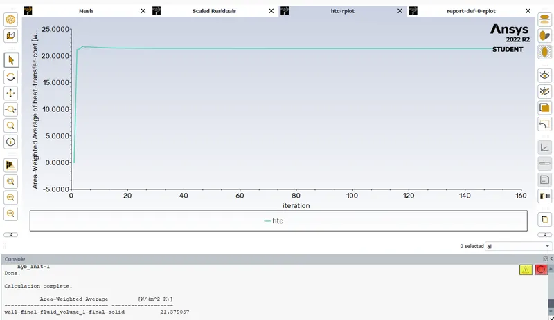
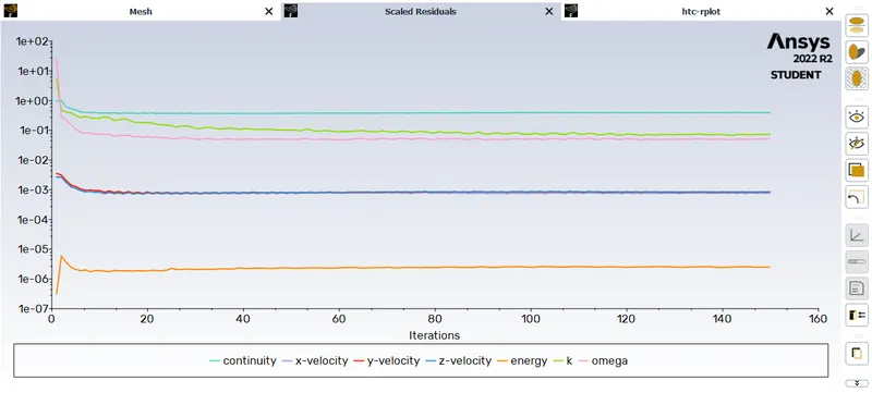
let us analyze above three models and the avg htc is come out to be 21.37 W/m2K

hence our base mesh is good and better we go further for next stage of solving and refer calculation as well

1. size = 90mm

first we need to find first layer height of inflation 

it is nothing but dy  we know that 

 Y+ = (dy x Uf x ρ)/μ

Uf - fric velocity

ρ density

we can take as y+ = 1 since for viscous sublayer 

hence Uf = (τ/ρ)^0.5

τ is wall shear stress

τ=0.5 Cf x ρ x v²

Cf is skin frictional coefficient

Cf= 0.0528 /Re^0.2

Re=ρ x v D / μ

by substituting known values

Re= (1.225 x 5 x 0.17)/(1.7894 x e-4) = 58189.9

Cf= 0.0528/58189.9^0.2= 0.00646

τ= 0.5 x 0.00646 x 1.225 x 5^2 = 0.0989Pa

Uf= (0.0989/1.225)^0.5 = 0.2841m/s

substituting known values in y+ eqn

1= dy x 0.2841 x 1.225/(1.78941 x e-5)

dy= 0.0514mm

hence dy is the first layer thickness

hence set mesh size for 90mm and perform simulation 

similiarly perform for 80 and 70mm 

they are as follows

 

 

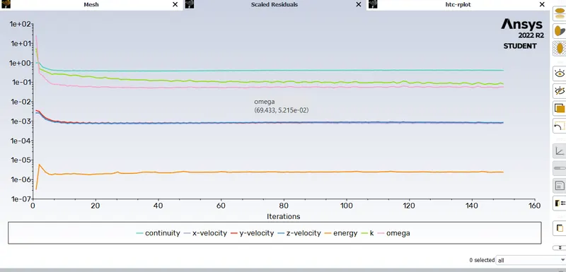
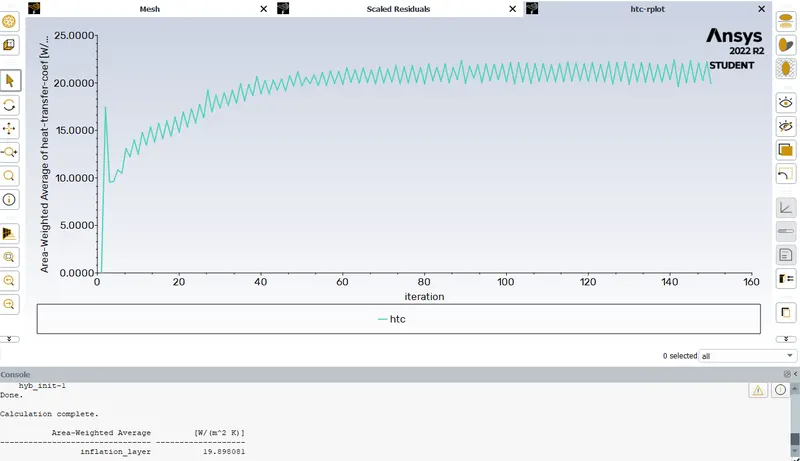
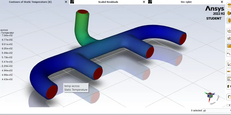
 80mm

 

 

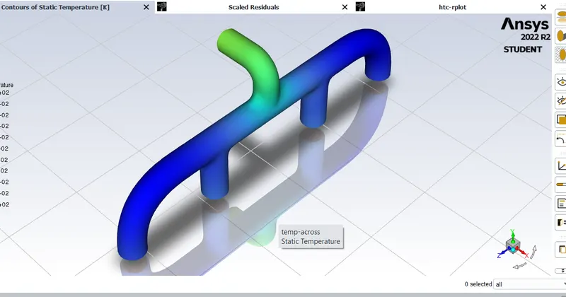
 70mm:

 

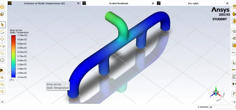
hence thus we simnulated three cases now we mathematically calculate HTC so that we can compare it to analytical values

we know

HTC = Nu x k / D

Nu = 0.023 x Re ^ (4/5) x Pr^n

Pr= μ x Cp/k

where 

Pr is prandtl no

k is thermal conductivity

by solving we get

Pr = (1.7894x e-5 x 1006.43)/0.0242

Pr= 0.74

NuD= 0.023 x (58189.9^0.8) x ( 0.74^0.3)

NuD = 136.26

HTC = (136.26 x 0.0242)/ 0.17

HTC = 19.39 W/m2K

Post processing:

we can see about plane analyzing

Results:

calculated HTC is   19.39 W/m2K

size	max size	no of elements	HTC	Deviation
90	100	257843	20.8	-1.41
80	90	267594	20.44	-1.05
70	80	278013	20.23	-0.84

hence avg deviation percentage is 5% from calculated value hence our simulation is correct.

Conclusion:

hence we done following in this challenge

performed simulation on different mesh sizes as 90 ; 80;70mm respectively

we maintained Y+ value throughout  inflation layer

we then calculated HTC mathematically and compared it with analytical values