Week 4 - CHT Analysis on Exhaust port

Aim

Perform Conjugate Heat Transfer Simulation in the exhaust port of engine with:-

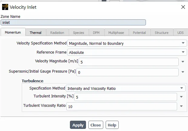
Inlet Vel = 5m/s

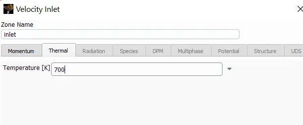
Inlet Temp = 700K

Introduction

The term conjugate heat transfer can be used to describe the processes which involve a temperature variation within the solids and fluids itself due to the thermal interaction between the solid and the fluid. During CHT the heat transfer can take place from solid media to the fluid media and vice-versa. This is because fluids flow around solids or between solid walls, and also the solids are mostly immersed in a fluid.

CHT analysis is beneficial in engineering applications because it shows the heat exchanging capabilities between the two surfaces in the engineering device and various optimization can be done to improve the thermal characteristics of the devices. Thus, this can be used to improve the heat transfer rate wherever required. It also helps us to identify the key parameters that enhance the fluid flow and heat transfer within the system.

CHT can be performed to improve the cooling performance of water jackets and increase the engine life.

Theory

CHT refers to the cases where the combination of heat transfer in solids and heat transfer in fluids is present. In solids, conduction dominates whereas in fluids convection is the primary mode of heat transfer.

For example, Heat Sinks are optimized to combine heat transfer by conduction in the heat sink with the convection in the surrounding fluid. Similarly efficiently combining heat transfer in fluids and solids is the key to design effective coolers and heat exchangers. In such devices fluid usually plays the role of energy carrier on large distances and solids play the role of separators in most of the cases so that the fluids exchange heat without mixing with each other.

Solving & Modelling approach

I have soved through the stages mentioned above with the help of videos shown and guidance of the technical staff.

The process fluesnt fluid flow will be done in following these 5 steps:-

1) Geometry - The geometry of the model will be formed where the actual flow will flow/interfere

2)Mesh - The meshing of the volume is done whoose parameters are set by default with help of 'Boundary Box'

3)Setup - The initial and boundary conditions or parameters and the model choosen are given to the model.

4) Solutions - Based on conditions and requirements the result is calculated with the help of model choosen

5) Results - The final results are appeared here from where the investigation of simulation is done.

Pre-processing and solver setting

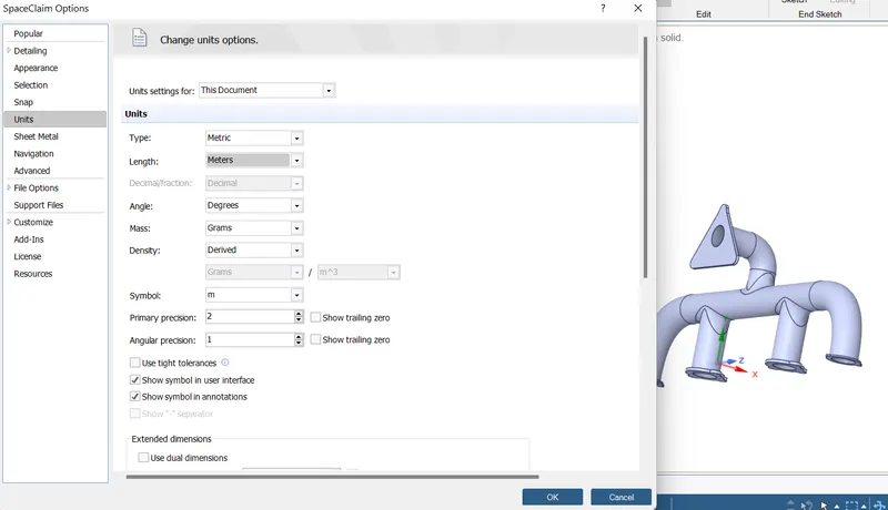
Step 0) Change unit to meters and import the downloaded geometry

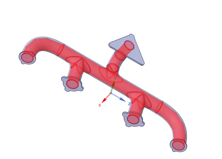
Step 1) The geometry was made as required.

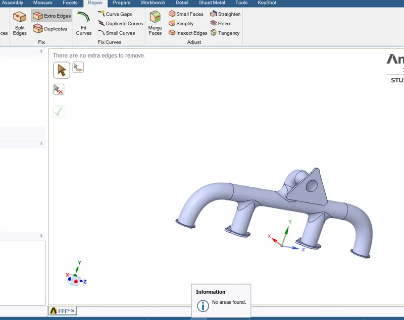
1.1) Repair of any extra edge found should be done

1.2) Extract the fluid volume from the solid volume and assign volumes their name

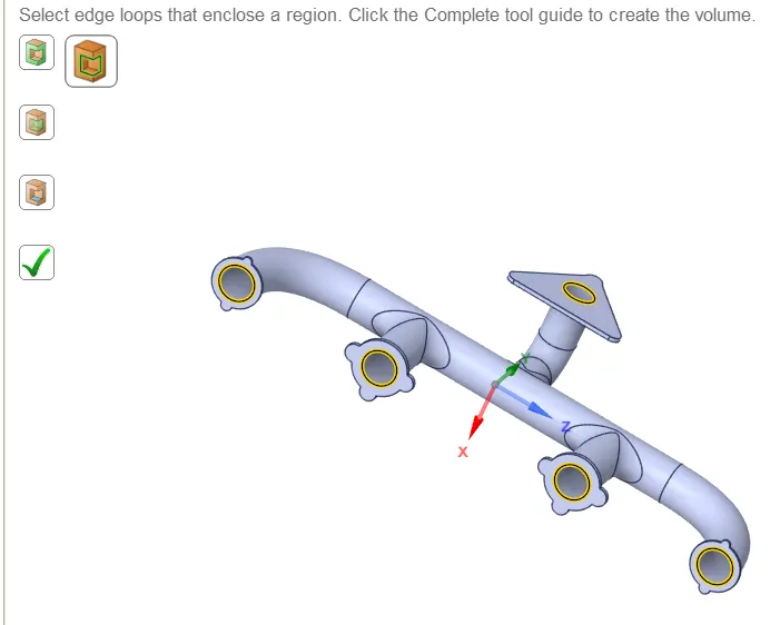
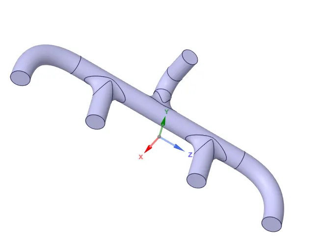
1.3) Make a common new component of the 2 and DELETE EMPTY COMPONENTS

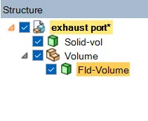
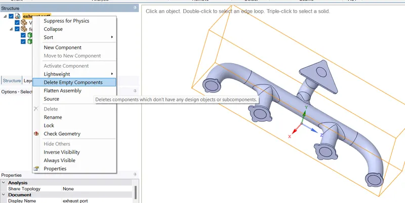
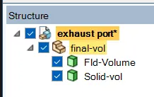
1.4) Make sure that the topos share with each other

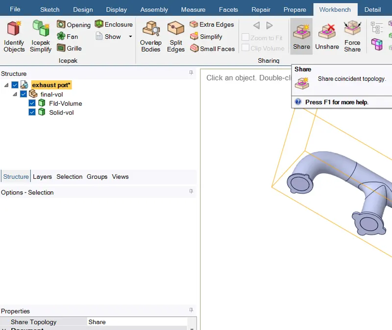
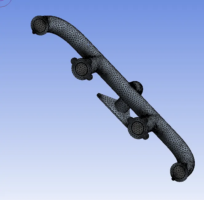
Step 2) Mesh the component.

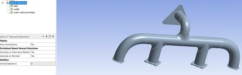
2.1) Assign names to the faces as requireed

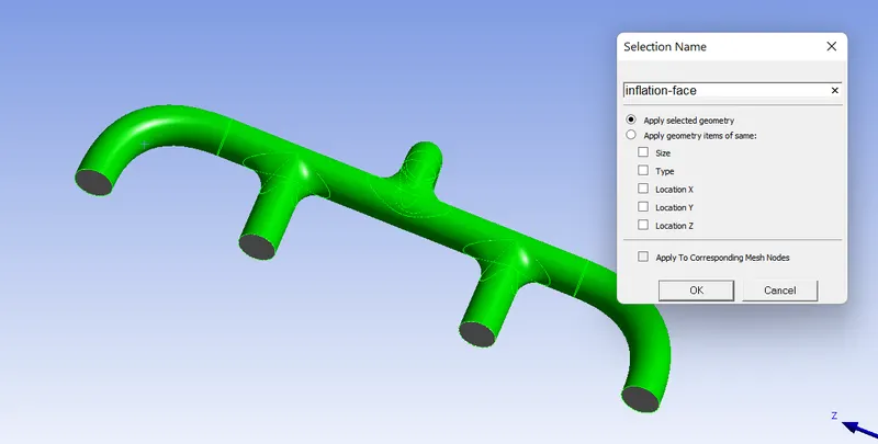
2.2) Give the setting to mesh for inflation

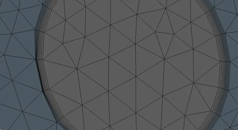
2.3) Give the settings of sizing to the mesh

Pre-processing and solver setting

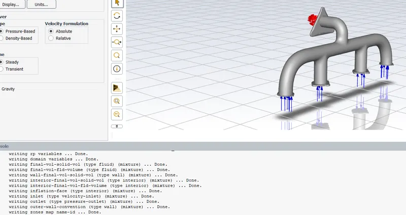
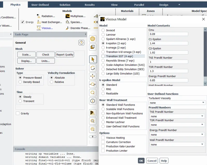
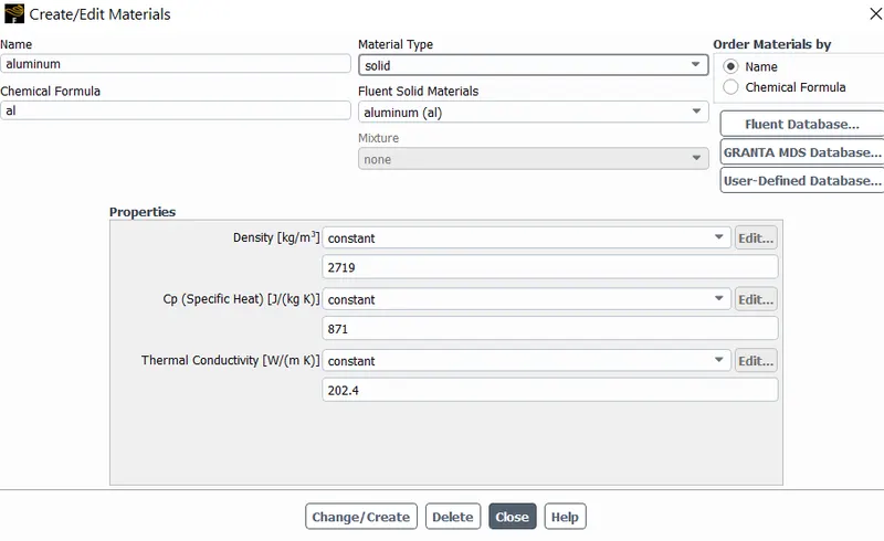
Step 3) Setup the system conditions and parameters.

3.1) Give the settings of physics as given below

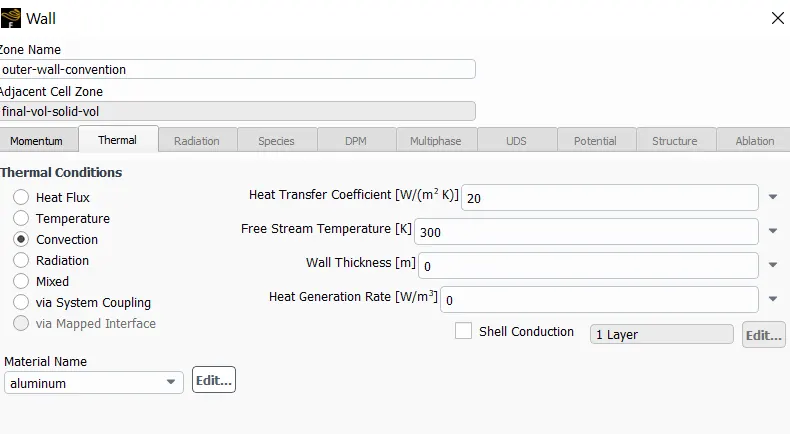
3.2) Give boundary conditoins to the system

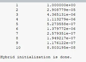
3.2) Hybrid initialize the system

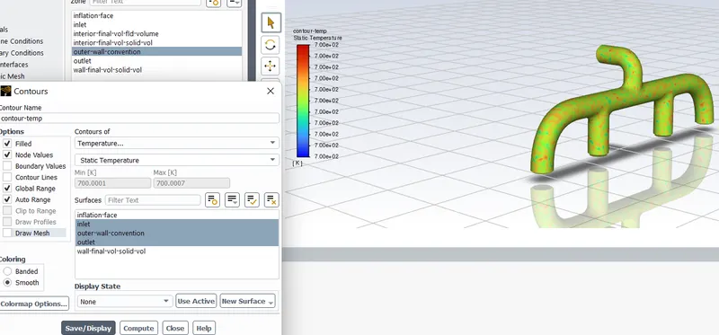
3.3) Give the contour for temp of system

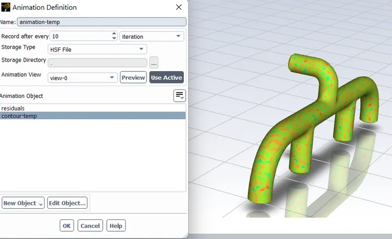
3.4) Create animation for simulation by providing the active view

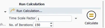
3.5) Calculate the result for 150 iterations.

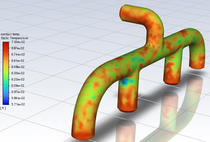
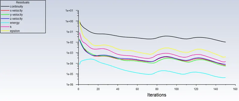
Step 4) Manupilate the result appearance as per our convinience

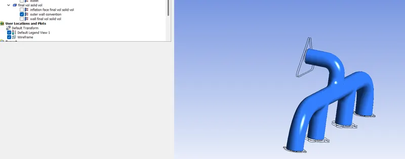
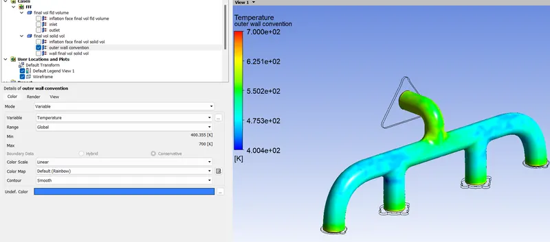
4.1) For the wall, increase transparancy and give variable color for the temperature difference

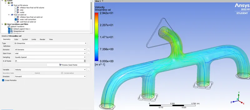
4.2) Add steamlines to the body

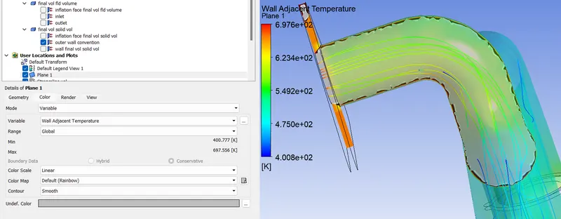
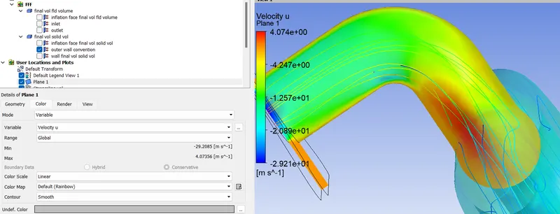
4.3) Insert XY plane to the body and give it's render as

1. Wall Heat Flux

2. Velocity in X-direction

Results

The simulation gives the following results:-

1. Iteration Convergence graph

2. Static temp contour

3. Velocity Steamlines

4. Wall Adjacent temp

5. Velocity of the fluid flow in plane view

Conclusion

Following points can be concluded from the report:-

1. The local temperature increases with increase of velocity

2. Velocity increases in the regions where inlets coverge and hence increasing the local heat tranfer co-efficient of the area.

3. The appeared results gets refined and more detailed with finer results.