Week 4 - CHT Analysis on Exhaust port
Aim:
The aim of the challenge is to calculate the wall/surface heat transfer coefficient on the internal solid surface and display the velocity and temperature contours.
Objective:
The main objective is to provide the following in the challenge report,
- Creating a brief description of why and where a CHT analysis is used.
- Calculate the wall/surface heat transfer coefficient on the internal solid surface & show the velocity & temperature contours in appropriate areas.
- verifying if the HTC predictions from the simulation are correct and predicting the factors that the accuracy of the prediction depends on.
Conjugate heat transfer:
Conjugate heat transfer (CHT) analysis can accurately predict heat transfer by simultaneously solving all the relevant solid and flow field heat transfer processes. The CHT approach has an advantage over FE thermal analyses in that wall heat transfer coefficients and their local variations on surfaces are directly calculated within the model rather than based on simplified empirical calculations.
Conjugate heat transfer corresponds with the combination of heat transfer in solids and heat transfer in fluids. In solids, conduction often dominates whereas, in fluids convection usually dominates.
Conduction: This is the transfer of heat through a solid. For example, heat generated inside an enclosure is transferred to the outer surface by means of conduction.
Convection: Convection is the transfer of heat from a surface by means of a fluid such as air. Natural convection occurs as air is heated: it expands, rises, and is replaced by cooler air. The amount of convection may be increased by using a fan to increase the flow of air.
Application of Conjugate heat transfer:
Conjugate heat transfer methods have improved as a modeling and investigational tool for natural phenomena and engineering systems in a variety of fields, including aerospace and nuclear reactors, thermal goods treatment, food processing, complex medical procedures, and ocean thermal interaction in metrology.
- Heat sinks are optimized to combine heat transfer by conduction in the heat sink with the convection in the surrounding fluid.
- The simulation of heat exchangers
- Cooling of electronic equipment
- General-purpose cooling and heating systems.
Procedure:
1. Import the geometry to SpaceClaim.
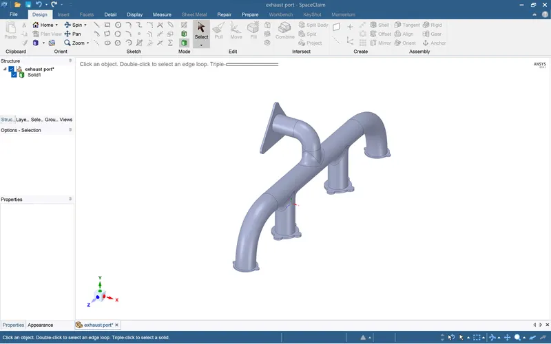
2. Using the repair option to delete the unwanted edges in the geometry.
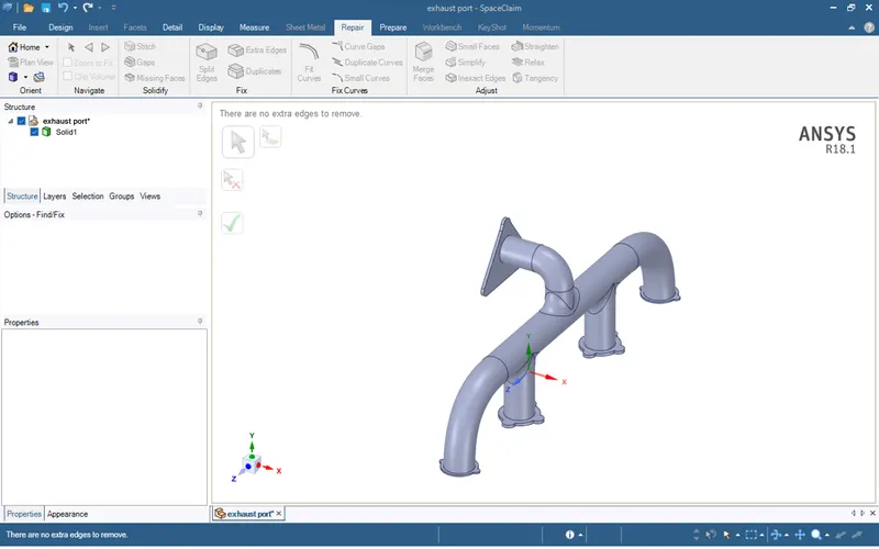
3. After repairing the extra edges extract the volume using prepare
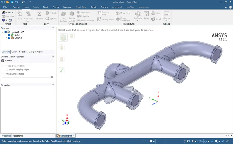
4. The solid and fluid volume is created and then meshing is done.
5. After importing name the sections.
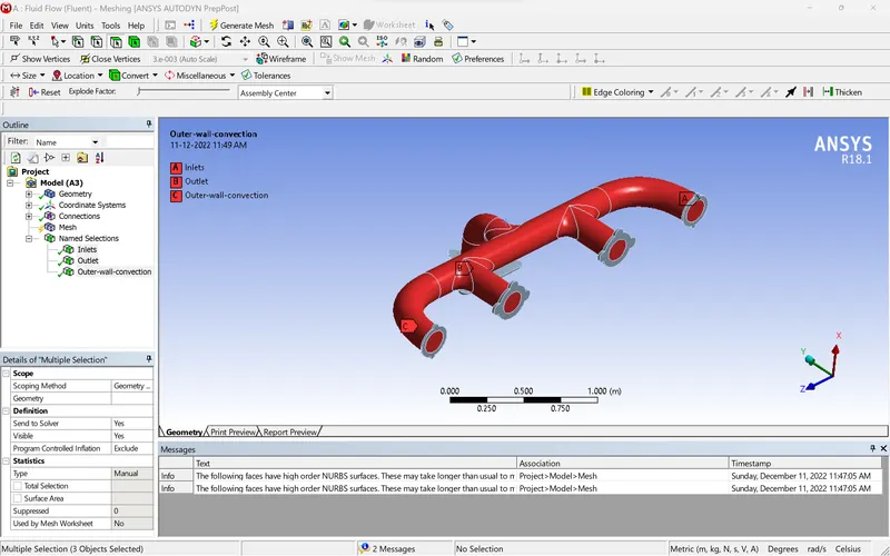
6. After the named section generate the mesh.
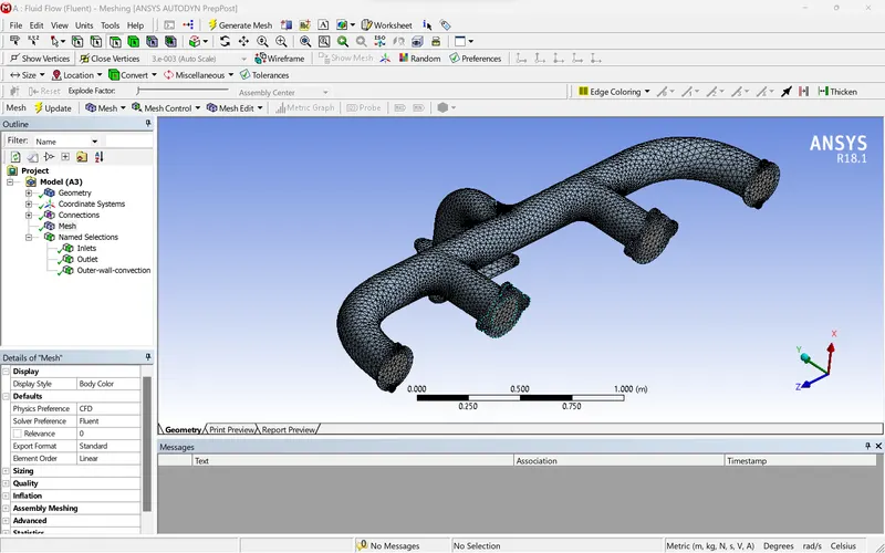
7. After the mesh is generated it is noted that there is no conformal mesh between the solid and fluid volume. To overcome this go to SpaceClaim and modify the geometry.
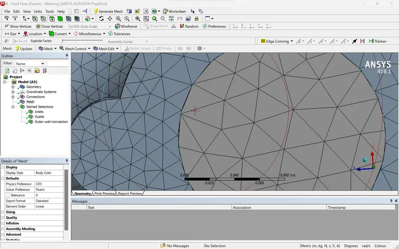
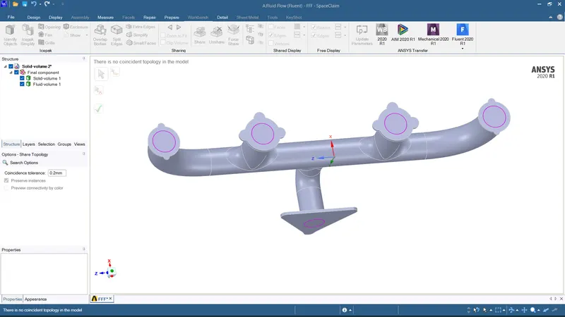
8. Close the mesh and open the SpaceClaim and generate the share prep to make interface between the solid and fluid surfaces.
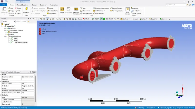
9. Again rename the sections in the model.
10. The share topology is shared between the solid and fluid volumes.
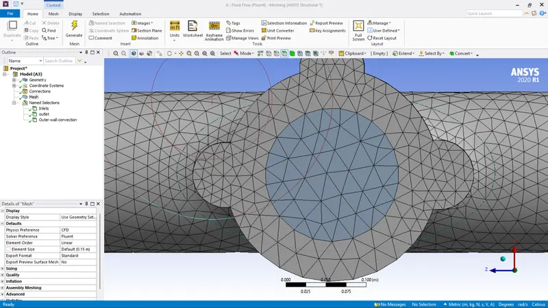
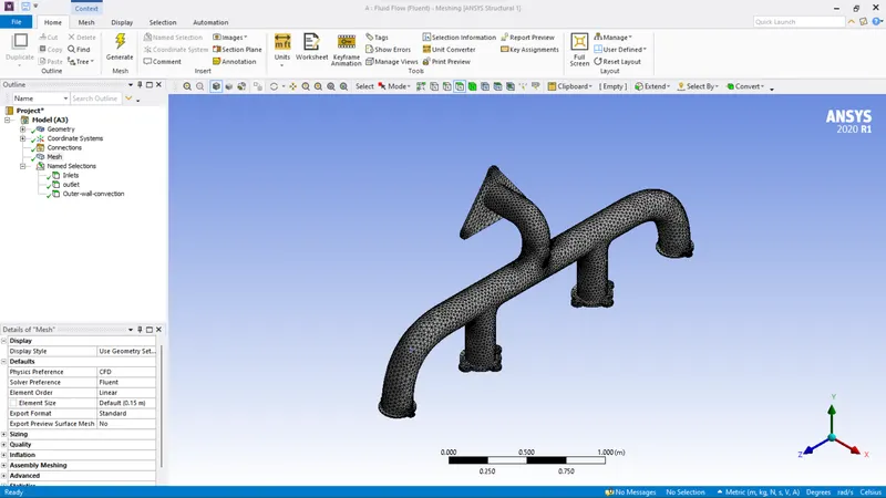
Case 1:
Mesh: Base mesh
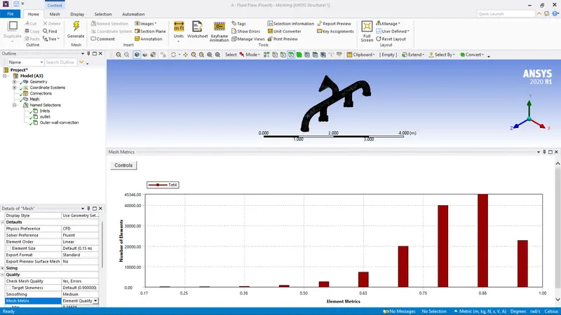
1. Element quality is given below.
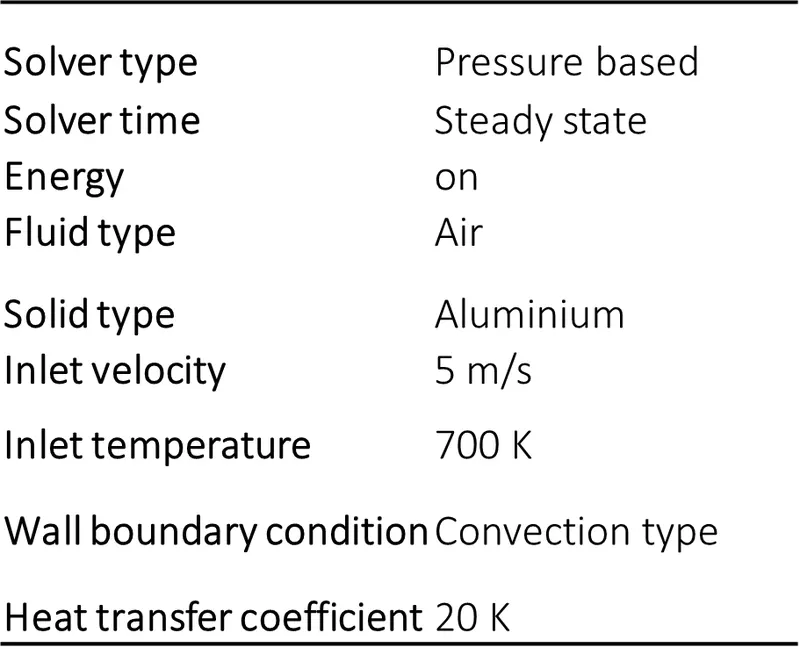
Below are the constraints given to the solver.
Air:
| Density | 1.225 kg/m3">m3m3 |
| Cp">Cp | 1006.43 J/kg K |
| Thermal conductivity | 0.0242 W/m K |
| Viscosity | 1.7894e-5 kg/m s |
Aluminum:
| Density | 2719 kg/m3">m3m3 |
| Cp">Cp | 871 J/kg K |
| Thermal conductivity | 202.4 W/m K |
2. Then go for the setup and start processing the solver.
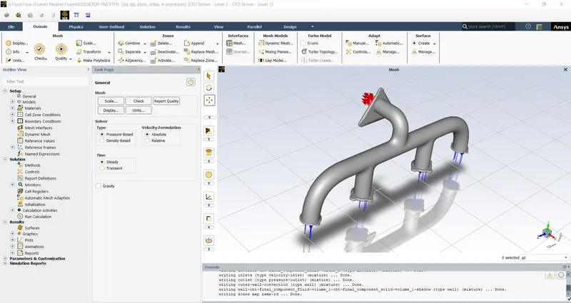
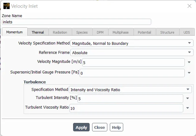
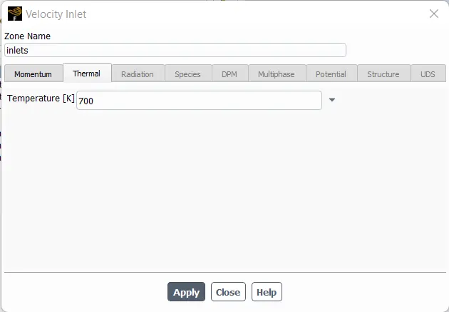
3. Inlet velocity and inlet temperature are given as 5m/s and 700 k.
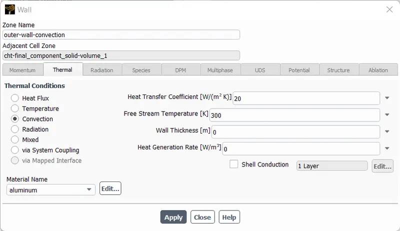
4. The wall constraints are given as convection and the heat transfer coefficient is 20 K.
5. Before initializing the setup provide the post-processing contour plots.
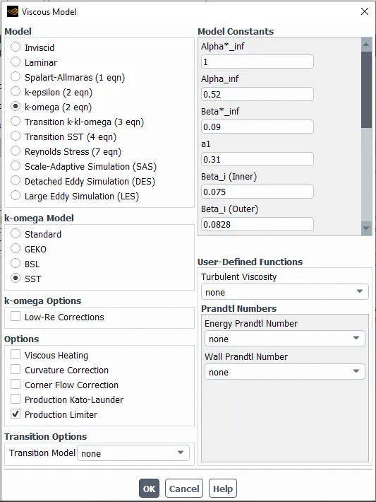
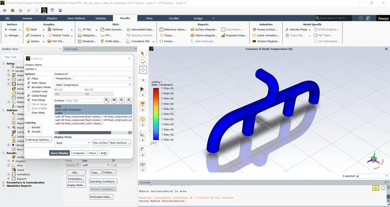
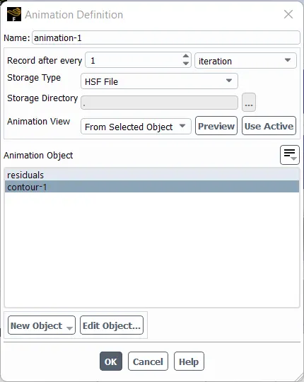
6. Animation setup is provided to visualize the temperature contour inside the exhaust port.
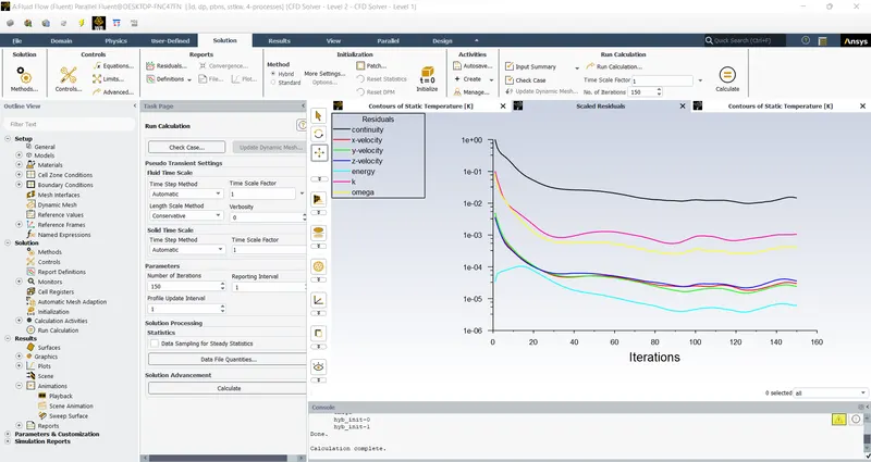
7. The residual plot of the solver.
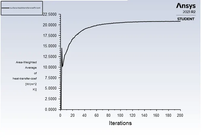
8. The surface heat transfer coefficient is,
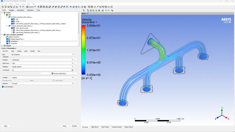
9. The streamline flow in the exhaust port.
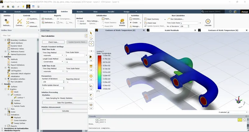
10. The temperature contour of the exhaust port,
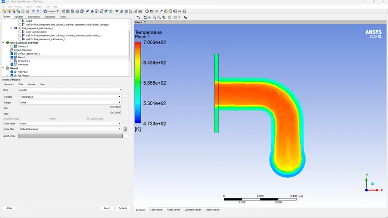
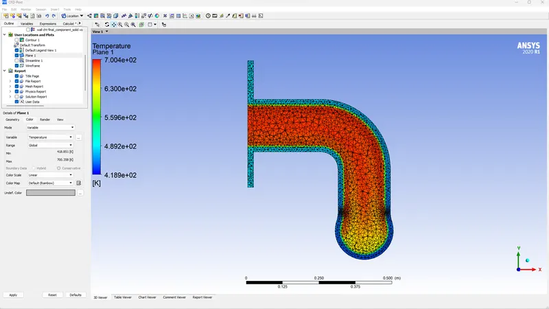
11. The plane is created in the XY and the themperature contour is shown below.
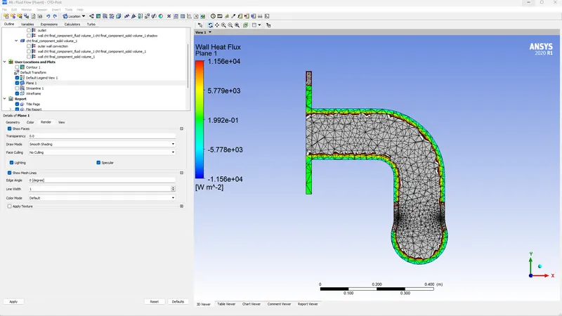
12. The wall heat flux in the plane XY.
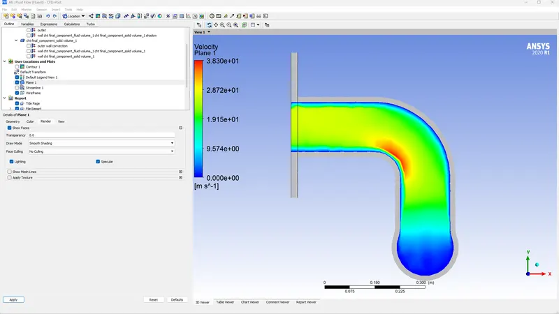
13. The velocity contour,
Case 2:
In this case,
Inflation thickness - 5mm
Mesh size - 50 mm
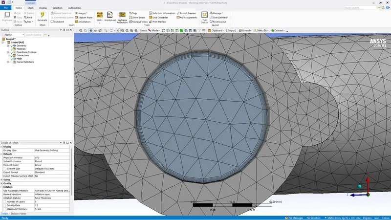
1. The 5 layers of inflation layer,
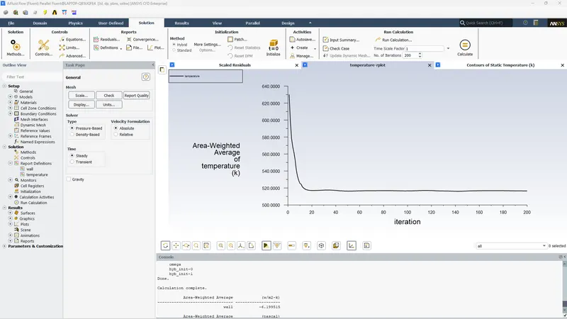
2. The Area-weighted average of temperature is,
3. The surface heat transfer coefficient for the mesh size 50mm is,
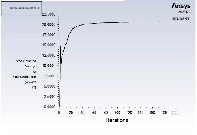
4. The wall heat flux in the first layer of thickness,
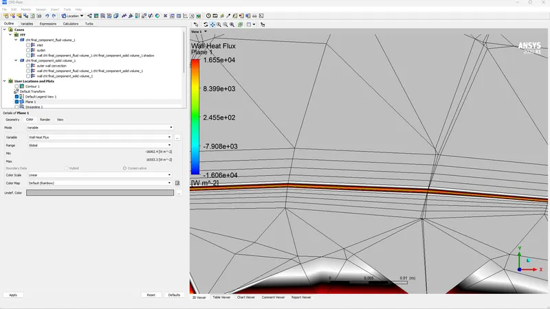
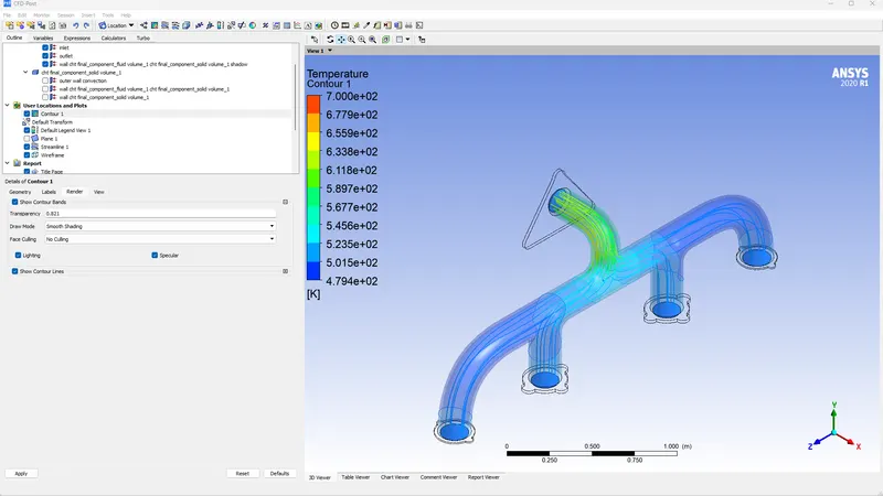
5. The temperature contour,
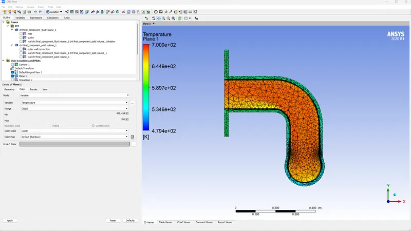
6. The velocity contour,
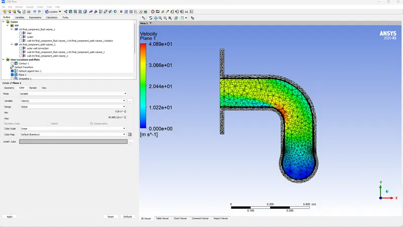
7. The streamline flow inside the fluid volume,
Case 3:
Inflation thickness - 0.06 mm
Mesh size - 10 mm
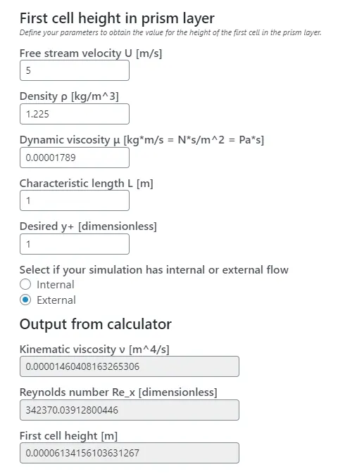
The generated fine mesh for the exhaust port is,
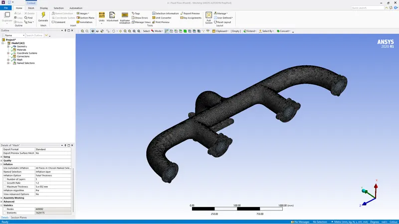
The Area Weight Average of temperature is ,
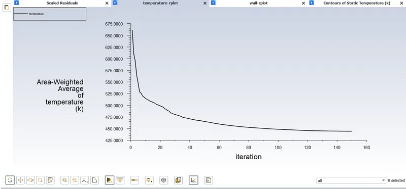
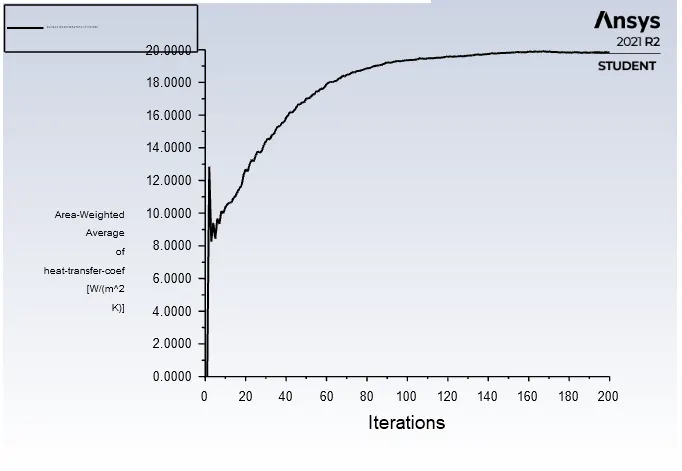
The Area Weight Average of heat transfer coefficient is ,
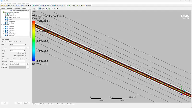
The first layer thickness of 0.06 mm of wall heat transfer coefficient is ,
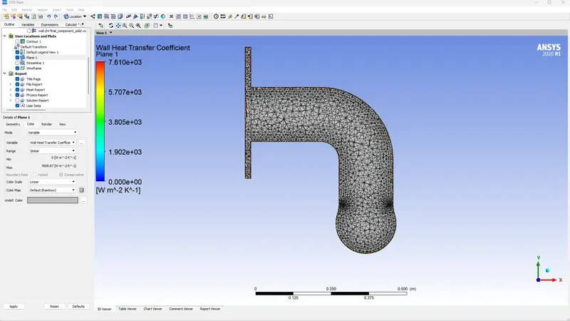
The wall heat transfer coefficient,
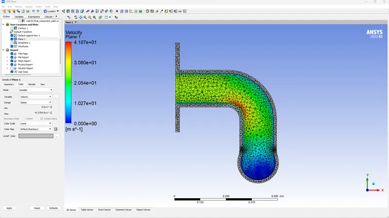
The velocity is,
The temperature is,
Conclusion:
1. HTC for the three cases is presented in this challenge.
Case 1: Base mesh - No inflation layer - HTC: 19.34
Case 2: Course mesh (50 mm) - Inflation thickness : 5mm - HTC :19.894
Case 3: Fine mesh (10 mm) - Inflation thickness: 0.06 mm - HTC:20.004
2. From the above table it is noted that the mesh is more fine the HTC will be accurate.
3. When we are using the finer grid by applying the inflation layer and reducing the element size to be nearly 10 mm we are getting the result with much less deviation.
4. The presence of the boundary layer is quite visible near the inlet of the wall where the velocity near the wall are to be close to be 0 to be the zero slip boundary condition so the viscous force is dominant near the inlet but near the outlet the velocity is the highest so giving the highest Reynolds number.
5. The value of the heat transfer coefficient is located in the call adjacent to the wall which allows allows us to choose the value of y+ = 1 for the turbulence model