Week 4 - CHT Analysis on Exhaust port

Aim:

1. To give a brief description of why and where a CHT analysis is used.

2. To Maintain the y+ value according to the turbulence model and justify the results.

3. Calculate the wall/surface heat transfer coefficient on the internal solid surface & also to show the velocity & temperature contours in appropriate areas.
4. To verify if the HTC predictions from the simulations are right? On what factors does the accuracy of the prediction depend on?

Introduction:The Conjugate Heat Transfer (CHT) analysis type allows for the simulation of heat transfer between solid and fluid domains by exchanging thermal energy at the interfaces between them. Typical applications of this analysis type exist as, but are not limited to, the simulation of heat exchangers, cooling of electronic equipment, and general-purpose cooling and heating systems.

Here we are considering exhaust port as an example for CHT analysis, the exhaust manifold is the key component in a 4-stroke IC engine. Exhaust manifold is mounted on the cylinder head of an engine. The exhaust manifold collects exhaust gases from multiple cylinders into one pipe. At the exhaust stroke the exhaust valve open and inlet valve remains closed that time piston starts moving from bottom dead centre to top dead centre sweeps out the burnt gases from the cylinders. These exhaust gases sweeps out from the cylinder and transfer through catalytic converter.One of the simplest ways to realize conjugation is through numerical methods. The boundary condition for the fluid and solid interface is set and solved through iteration methods. There are no right guesses for the values of the initial boundary condition for the convergence except through the hit and trial method.

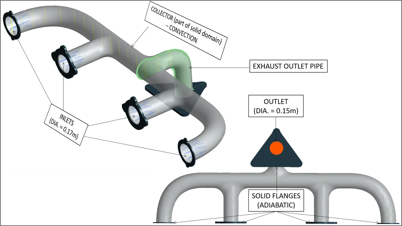
The CHT approach has an advantage over FE thermal analyses in that wall heat transfer coefficients and their local variations on surfaces are directly calculated within the model rather than based on simplified empirical calculations. The CHT approach therefore has benefits for those applications where heat transfer is either non-uniform or difficult to calculate empirically.

Applications:

Effective heat transfer: combining heat transfer in fluids and solids Efficiently is the key to designing effective coolers, heaters, or heat exchangers.The fluid usually plays the role of energy carrier on large distances. Forced convection is the most common way to achieve a high heat transfer rate. In some applications, the performances are further improved by combining convection with phase change (for example liquid water to vapor phase change). Even so, solids are also needed, in particular, to separate fluids in a heat exchanger so that fluids exchange energy without being mixed.

Procedure:

step 1:

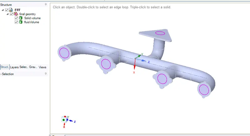
• import the geometry into space claim and check the units.

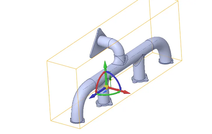
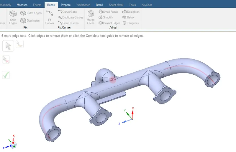
• Remove the extra edges in the model.

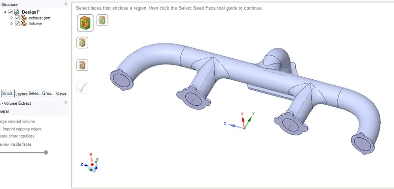
• Then perform volume extraction in the model and name the inner volume as fluid and outer volume as solid volume and remove the empty components.

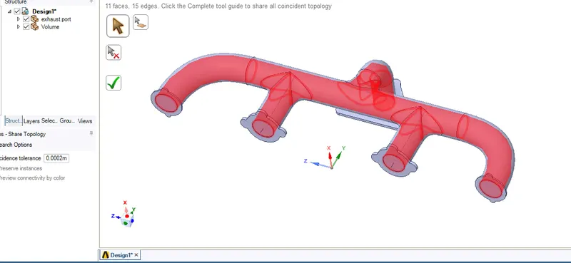
• click on Share topology of the component so that the mesh and physics information can be shared and conformal mesh can be achieved.

step 2:

• once geometry setup is done, exit SpaceClaim and open the mesh in workbench.
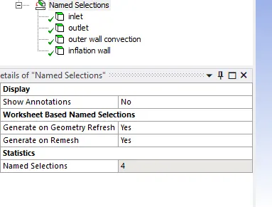
• select the faces and create name selections accordingly

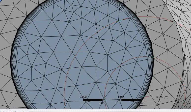
• generate the mesh in order to see the number of elements and nodes with default parameters without inflation layers, then refine the mesh with element size = 0.095m, aslo we need to see the things that needs to be refine since in CHT analysis we are interested at the interface betwen solid and fluid medium, so let us create inflation layer at the interface

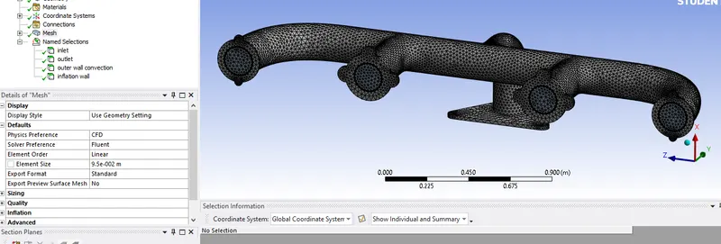
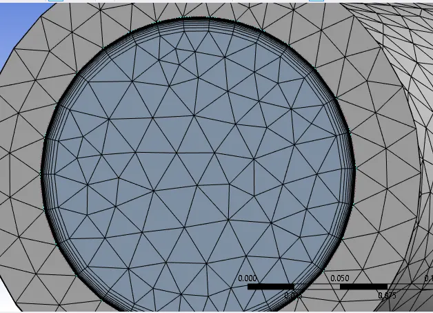
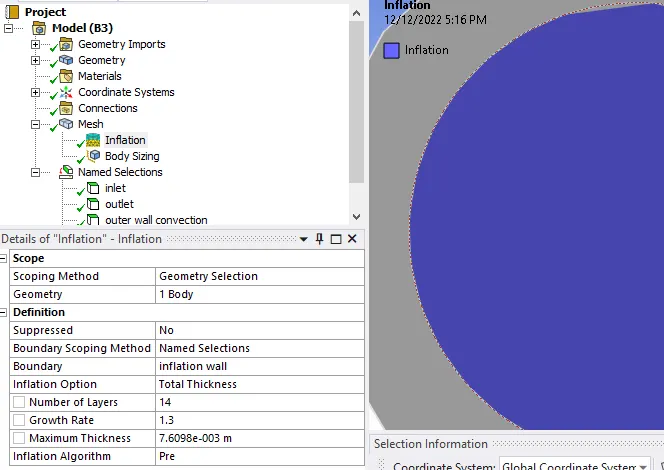
first and total layer thickness is calculated using the y+ calculator and checked whether the total prism layer thickness is almost equal to boundary layer thickness and created at the model.

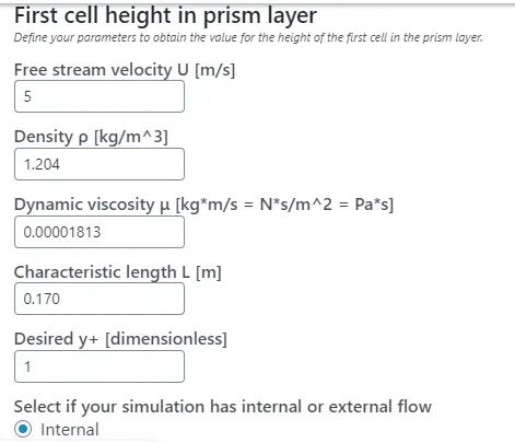
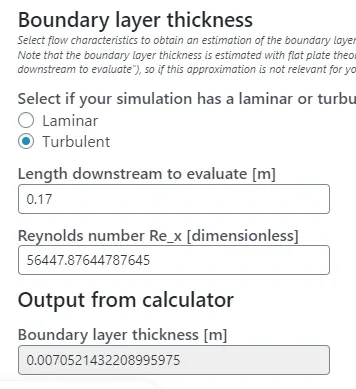
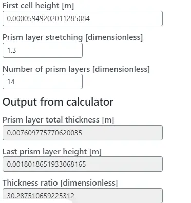
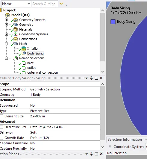
• Create a body sizing on the outer wall convection to achieve mesh refinement and accurate results can be captured at such regions.

step 3:

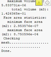
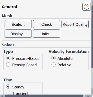
• After updating the mesh open setup(fluent), perform mesh check, select a pressure-based solver ->steady-state time simulation->absolute velocity under the general settings.

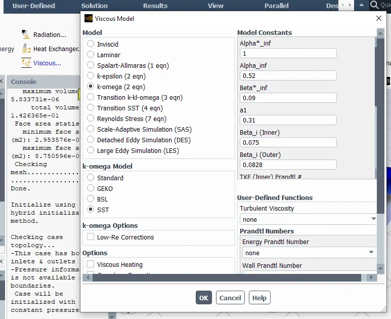
• Under physics click on the energy option since we are dealing with temperature and we are using k-omega SST model since we are interested the analysis near the wall.

• Input the Boundary conditions at the inlet=5 m/s as inlet velocity at temperature=700k and outer wall convection boundary to convection type and input the heat transfer coefficient as 20 W/m^2 K. and under cells check and update the type of volume for solid and fluid surfaces.
• Under materials, properties choose air as the fluid material and aluminum as the solid material.

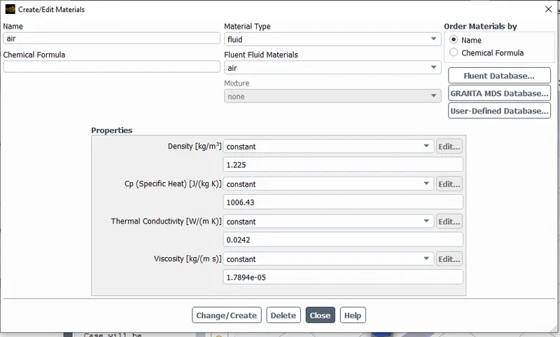
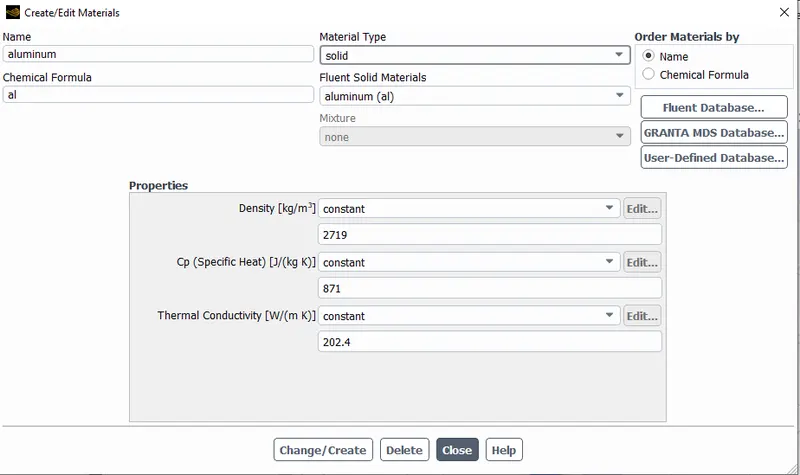
• Enter the reference values as per the geometry and inlet boundary conditions accordingly.

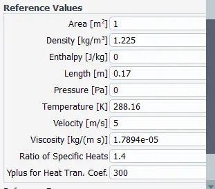
• create report for total heat transfer coefficient and contour for temperature to see how heat transfer is happening.
• Initialize by using the hybrid initialization, and the simulations for 300 iterations as it is optimum to achieve a converged solution.

Results:

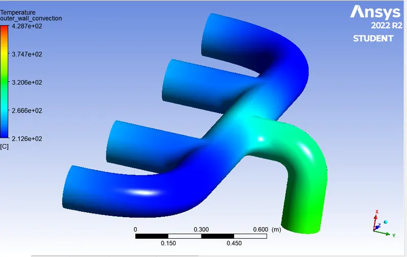
case 1:

inlet velocity=5m/s

outlet gauge pressure: 0 Pa

outerwall convection- type: convection;h=20W/m^2 K.

number of mesh elements :309454

number of node elements : 107557

no of inflation layer=10 with total thickness of 6.85519351859821E-03

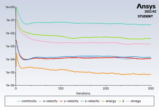
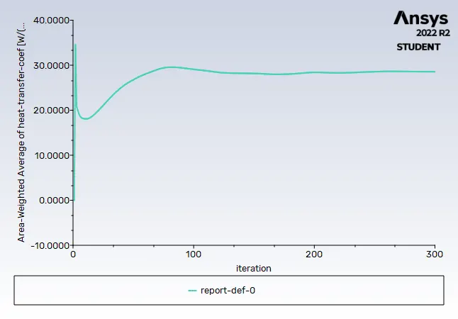
residuals area-weighted avg of heat transfer coefficient=28.5526

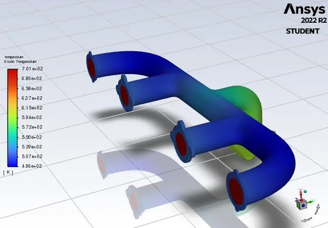
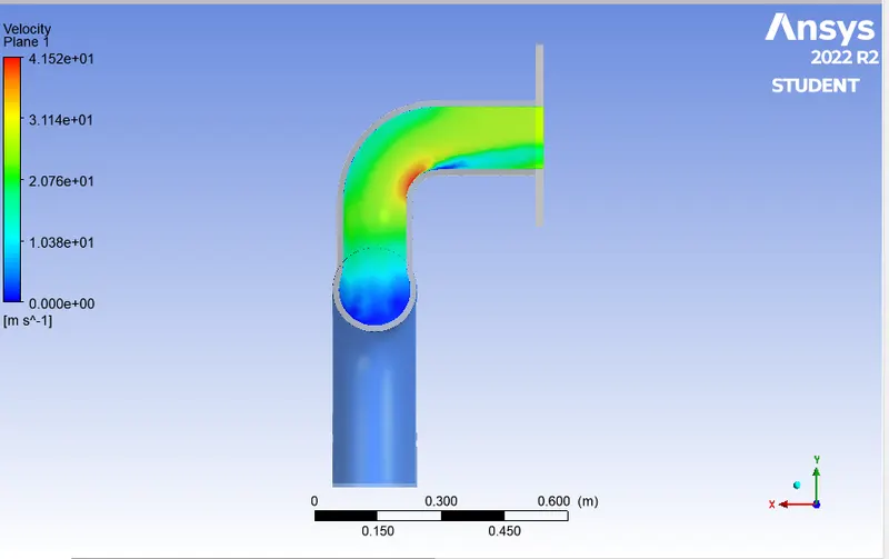
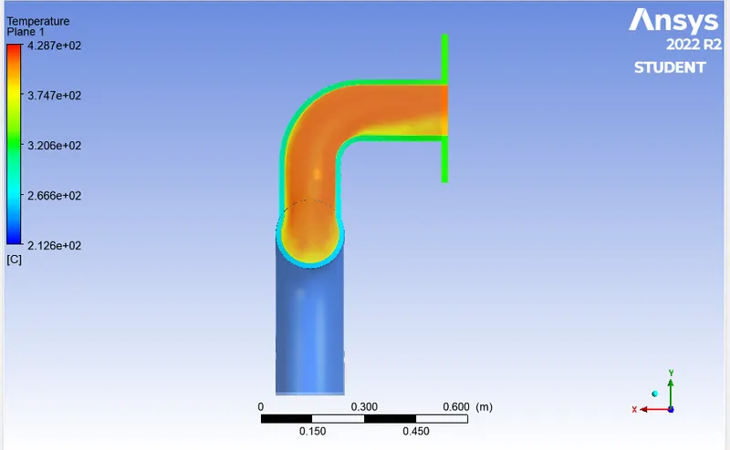
Temperature distribution velocity contour

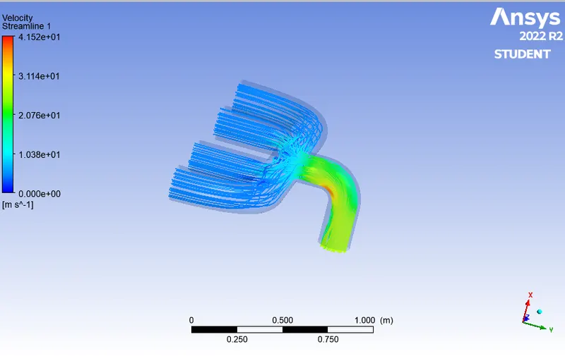
Temperature contour velocity streamline

case 2

inlet velocity=5m/s

outlet gauge pressure: 0 Pa

outerwall convection- type: convection;h=20W/m^2 K.

number of mesh elements :375417

number of node elements : 139238

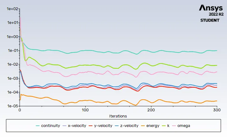
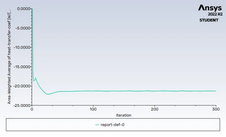
residuals area-weighted avg of heat transfer coefficient=-21.0978

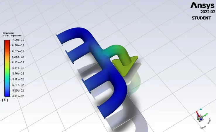
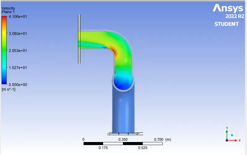
Temperature distribution velocity contour

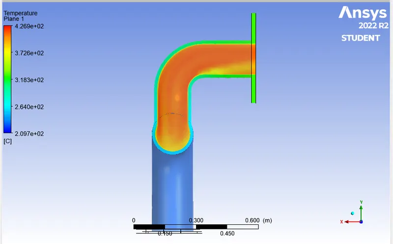
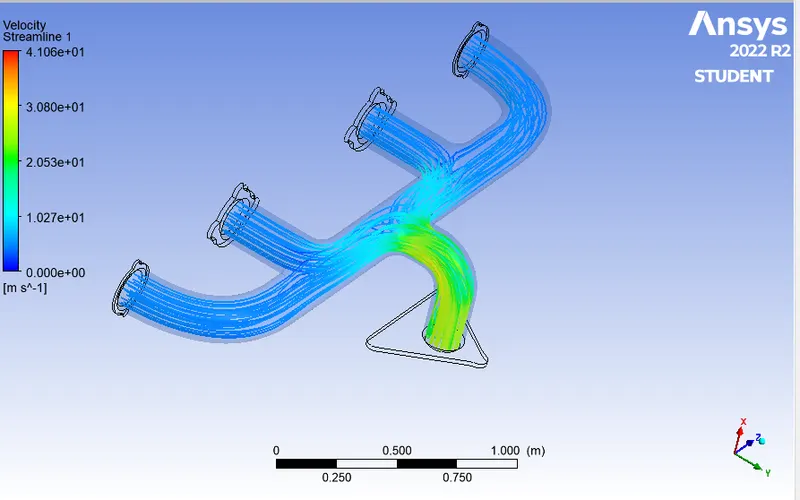
Temperature contour velocity streamline

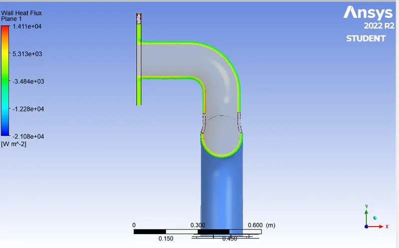
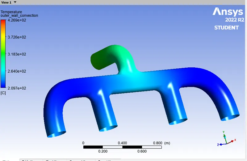
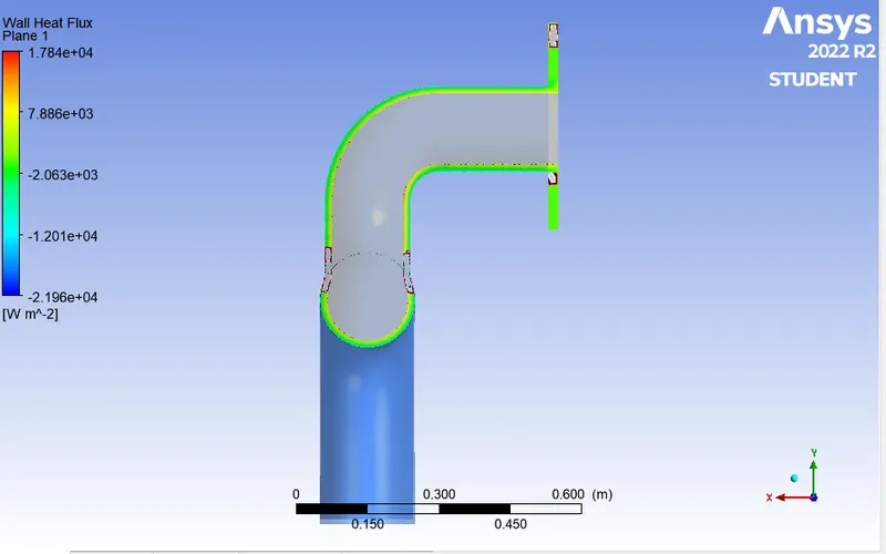
In the above analysis from case 2, we can see that the heat transfer coefficient obtained is of h = -21.0978 w/m^2-k and also CFD will create two surfaces name & name shadow,Both lie on the same surface. Only the direction changes i.e. signs, For the case 2 & 1, heat is rejected from fluid to the pipe wall. I.e. HTC = -21.5 W/m2K.

1) Analytical solution:

The Reynolds number of the flow is of Re = 56447.8764 with considering the flow velocity = 5 m/sec

we will use Dittus-Boelter equation for calculating heat transfer coefficient the formule follows as below,

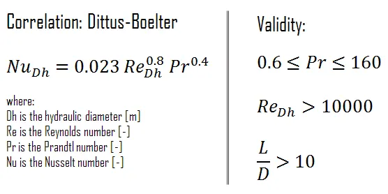
Nu(D) = 0.023* Re^(0.8)*Pr^n here n = 0.4 . D = diamter of the pipe = characteristics length = 0.17 m

the prandtl number is of the following

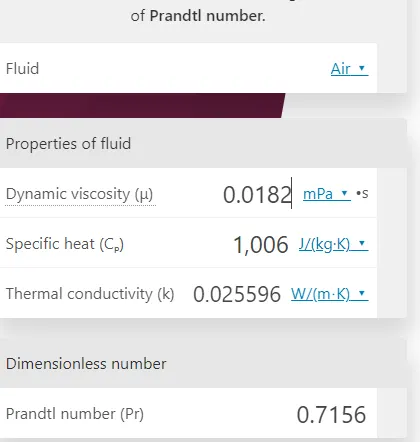
Pr = C_pμ/k here μ = 0.0182 mpa cp = 1006.43 J/kg-k and k = 0.025596 w/mk

∴ pr = 0.7156

the Nusselt number is calculated as Nu = 0.023*56447.8764^(0.8)*0.7156^0.4 = 127.3250

Nu = hL/kf = 127.3250 = h*0.17/0.025596

so h = 19.17065 W/m^2 K.

factors at which the accuracy of the prediction depend on

• From the theoretical value=h = 19.17065 W/m^2 K. we can see that the value is really close to the the computational value of the surface heat transfer coefficient h= 21.0978 W/m^2-K.
• The deviation of numerical heat transfer coefficient values from the analytical solution was found to be within 10% for the used mesh refinement and these are found to be in agreement with the industrial standards.
• When mesh refinement is done with inflation layer from the less refined mesh we can see that the deviation of 'h' is less compared coarse mesh.
• The velocity at the outlet is high than in the inlet this can be attributed to one outlet and the four inlets.
• The value of the y+ is maintained at 1 for the turbulence model since we are using k-omega turbulent model to solve(from reynolds number). This is validated with the analytical solution to compare with computational value and it was found out that The value of the heat transfer coefficien is found out to be 21.0978 W/m^2 K. which is approximately close to the analytical value.
• Since we are conducting CHT analysis at the interface it is very important as we want capture all the elements at that region, we are creating a structured inflation layers so that flow is captured and analyzed.

Conclusions:

1. Geometry preparation in Spaceclaim - Extra edges, Fluid volume extraction, share topology were learnt and understood.

2. The CHT analysis on the exhaust port was simulated and observed.

3. High-temperature concentration zone predicted and observed.

4. Comparison between the solver models for accurate results were done and checked.