Week 4 - CHT Analysis on Exhaust port

• CHT Analysis on Exhaust port
• Objectives:
  1. Give a brief description of why and where a CHT analysis is used.
  2. Maintain the y+ value according to the turbulence model and justify the results.
  3. Calculate the wall/surface heat transfer coefficient on the internal solid surface & show the velocity & temperature contours in appropriate areas.
  4. How would you verify if the HTC predictions from the simulations are right? On what factors does the accuracy of the prediction depend on?
• Conjugate heat transfer
• Heat transfer coefficient
• Give a brief description of why and where a CHT analysis is used.
• It is a heat transfer analysis between solids and fluids.
• This type of heat transfer includes both convective (liquid-to-liquid) and conductive (solid-to-solid) heat transfer, and both forced and natural convection.
• The heat transfer simulation type allows you to calculate temperature distribution and heat flow in solids subjected to thermal stresses (such as convection and radiation).
• A convective heat transfer analysis can be used when the temperature of a liquid changes its density.
• Typical applications for this type of analysis include heat exchanger simulation and electronic device cooling,Purpose cooling and heating system.
• Conductive heat transfer is heat transfer due to molecular excitation within a material without bulk mass transfer.

• Dittus Boelter equation
• This correlation is the so-called Dittus–Boelter correlation given as. Nu DB = 0.023 Re 0.8 Pr 0.4.
• Reynolds number

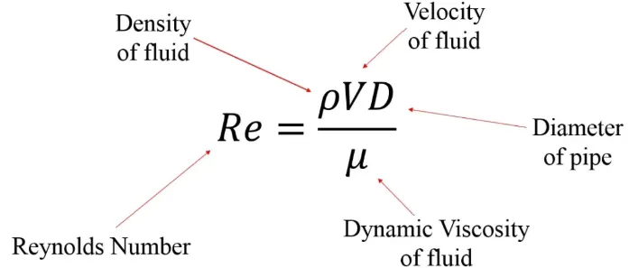
• Prandtl number

where, = Prandtl number

= momentum diffusivity

= thermal diffusivity

• Nusselt number

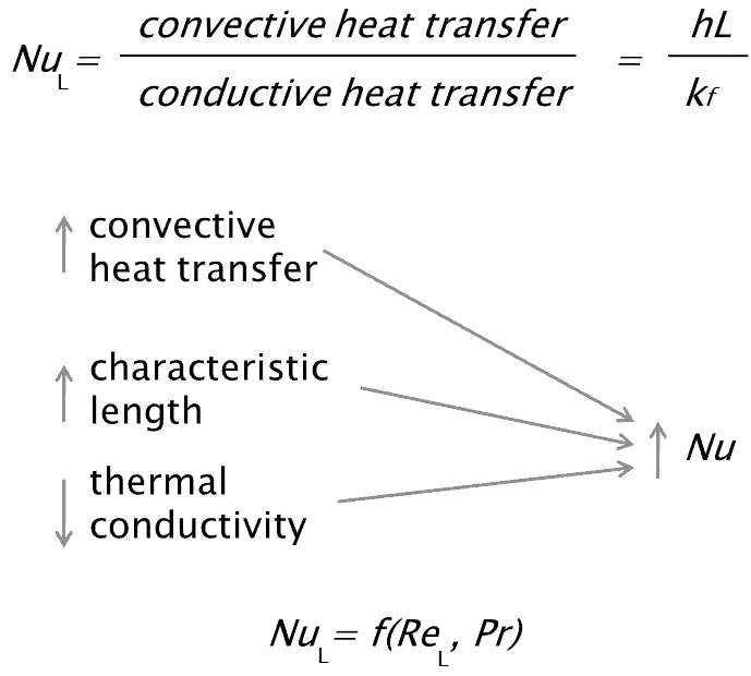
• Heat transfer coefficient

where , h = heat transfer coefficient

= Heat flux

= difference in temperature between a solid surface and surrounding fluid

• Procedure
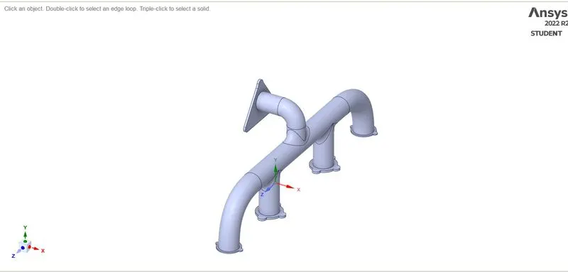
• Geometry imported in spaceclaim

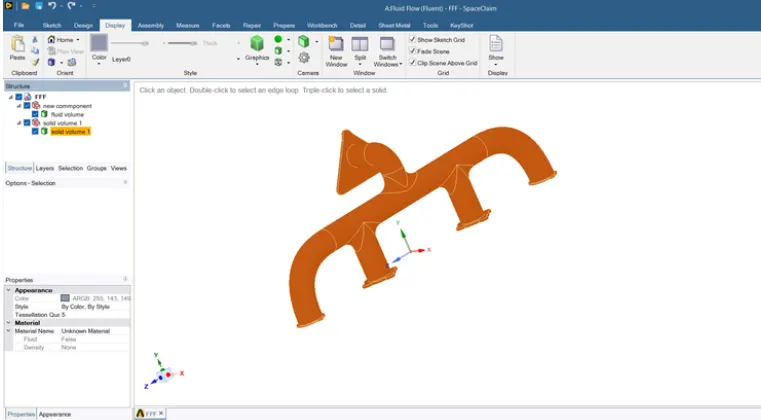
• Volume Extraction tool is used

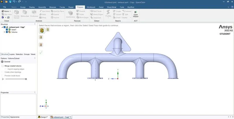
• The solid volume is created

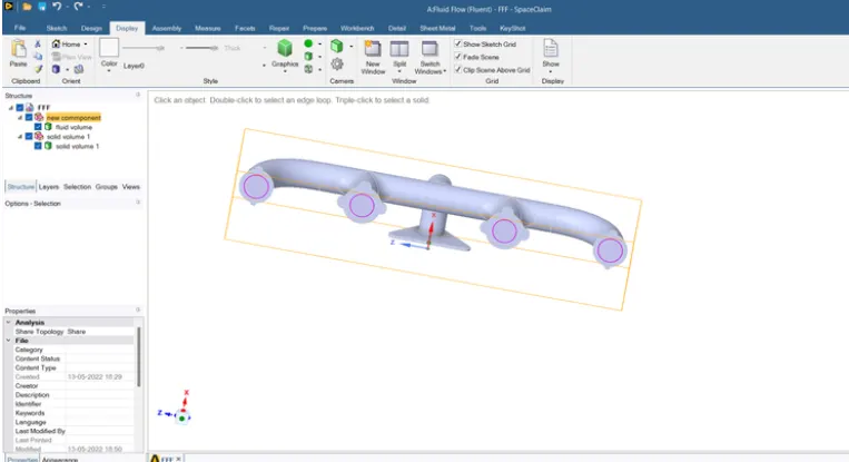
• The solid and the fluid volume is created

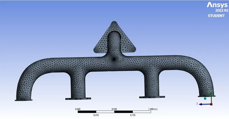
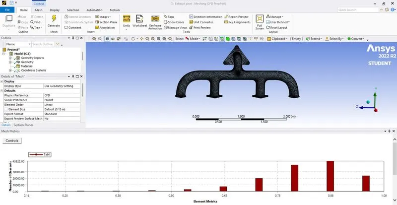
• Baseline mesh

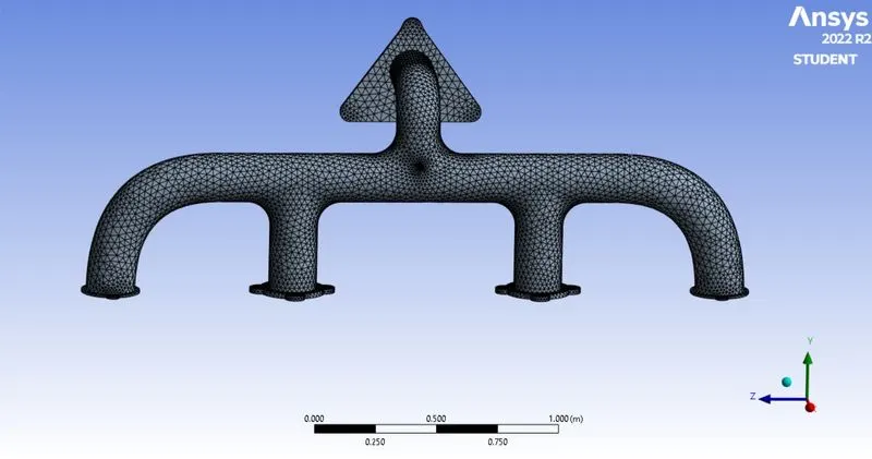
• Refined Mesh

• Mesh metric

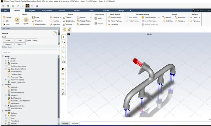
• Imported in fluent

• Material properties-

  Fluid -

  Fluid name = air.

  Density = 1.225 kg/m^3

  Specific heat = 1006.43 J/kg-k

  thermal conductivity = 0.0242 w/m-k

  viscosity = 1.789e-5 kg/m-sec.

  Solid -

  the solid material is of aluminum

  Specific heat = 871 J/kg-k .

  Thermal conductivity = 20 w/M-k

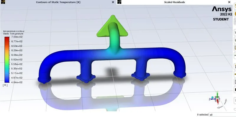
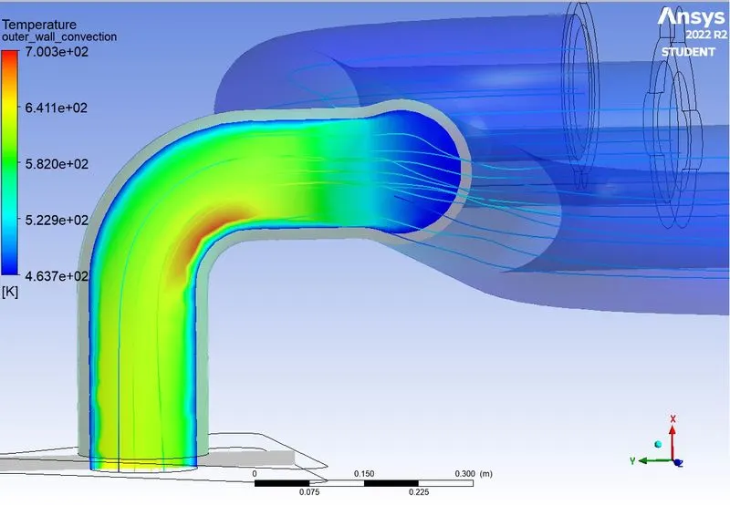
• The temperature contours

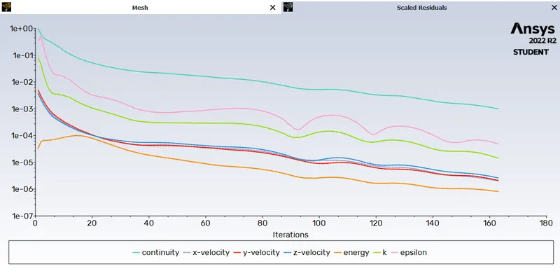
• Residual plot

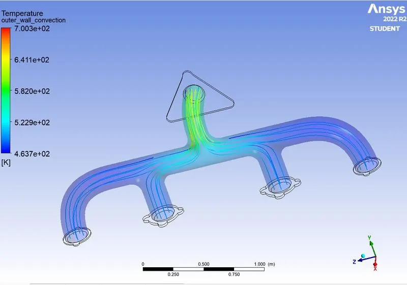
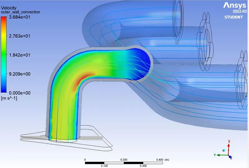
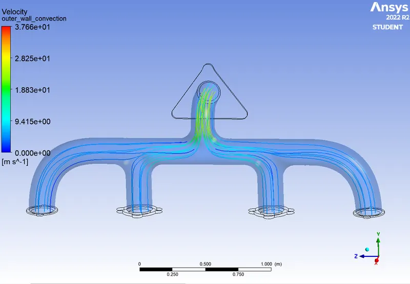
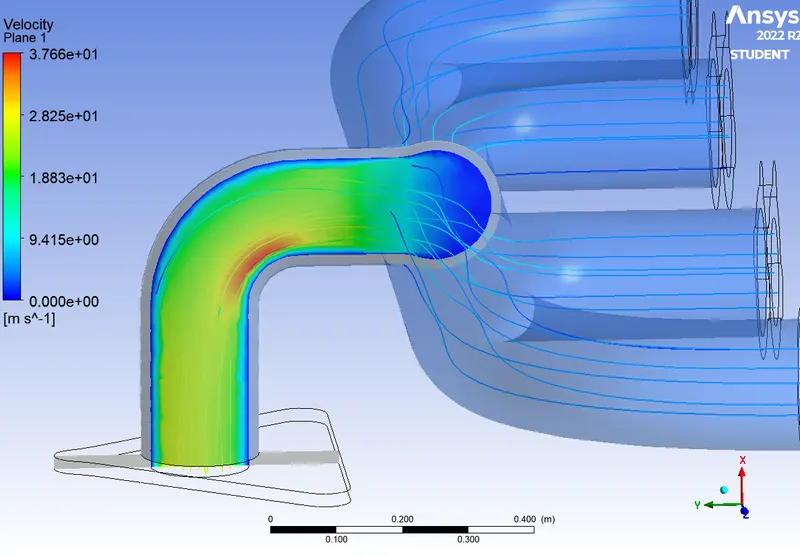
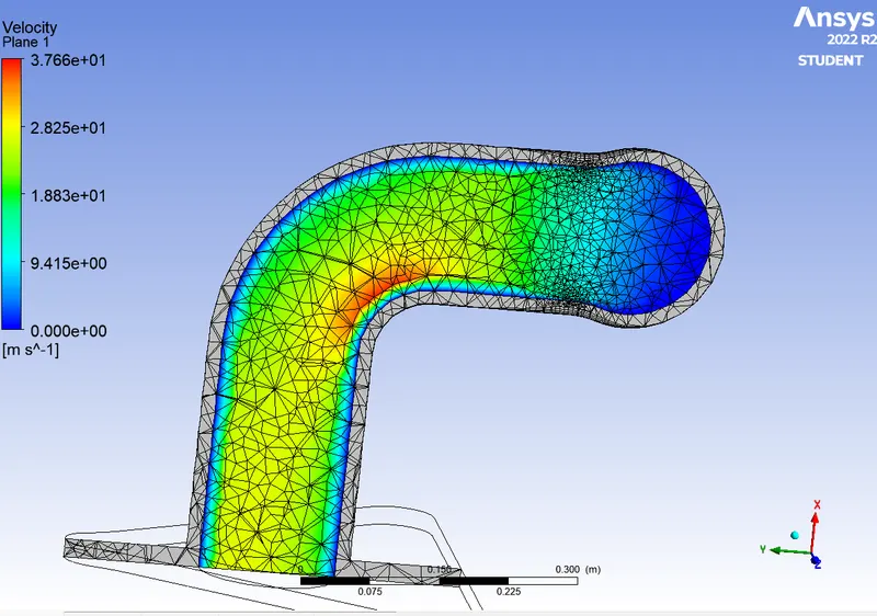
• Velocity and temperature contour for outer wall convection

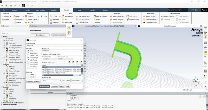
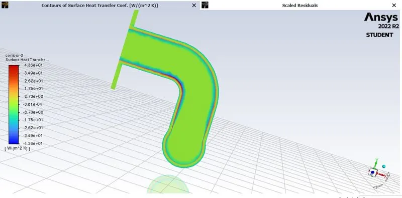
• Heat transfer coefficient plot

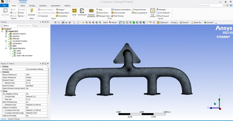
• case 2 ) In these the inflation layers are added and the element size of the solid surface mesh is also reduced further to 10 mm size-

  The Inflation layer is added to the geometry 6 layers are added

  Growth rate = 1.2

  Number of inflation layers = 6

  First layer thickness = 0.0514 mm

  captured curvature is set to yes.

• Mesh

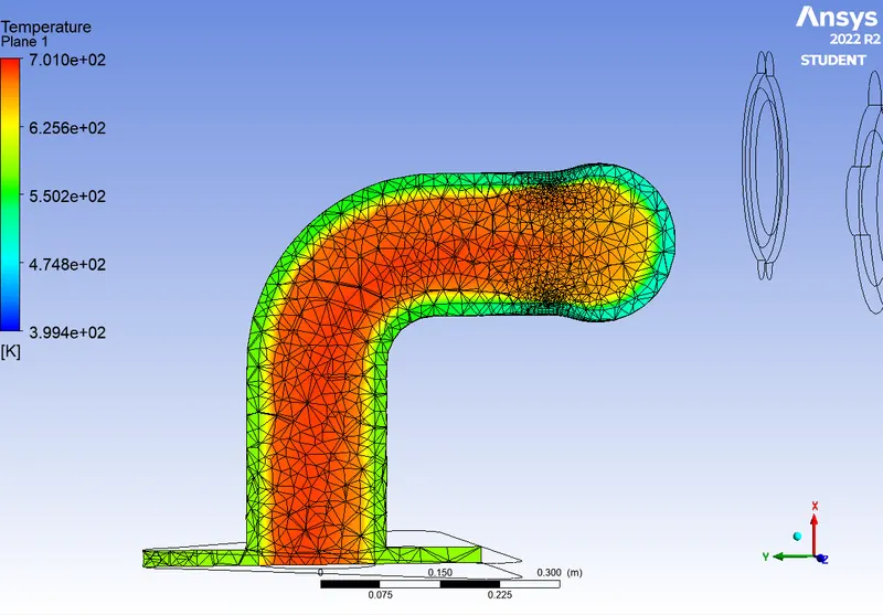
• Temperature contour

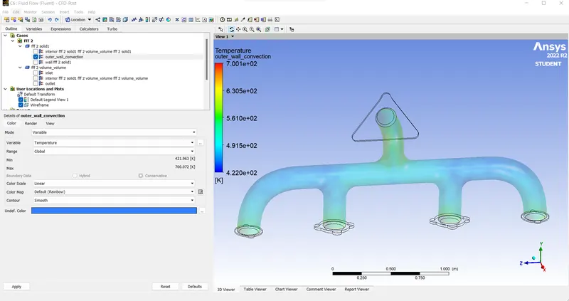
Temperature = 700k

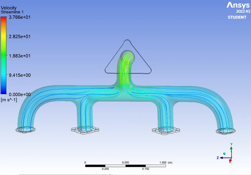
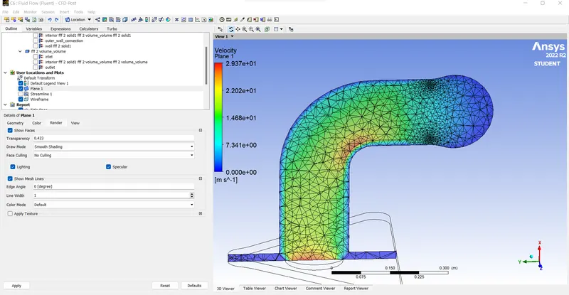
• Velocity contour

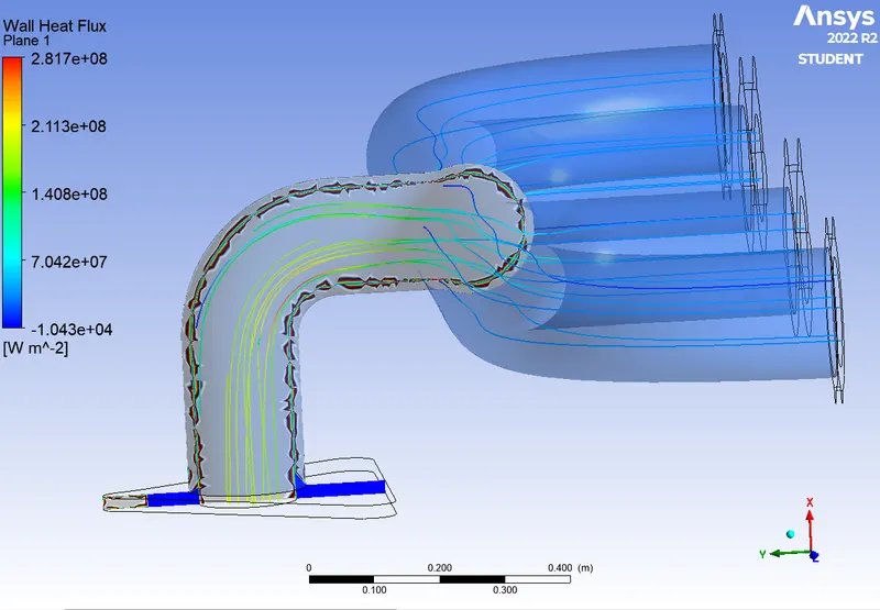
• Wall heat flux

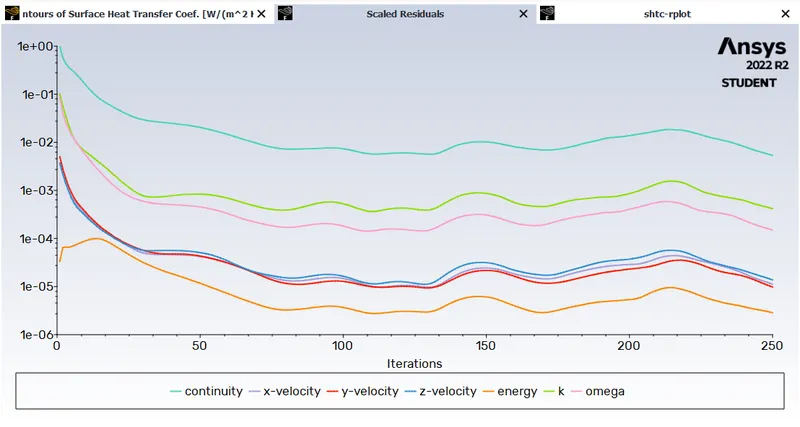
• Residuals

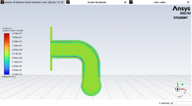
• Heat transfer coefficient plot

• Stepwise explaination
• The exhaust pipe was modeled in the space claim.
• The exhaust port is a three dimensional model containing four inlets and one outlet.
• Despite having the isothermal boundary condition and a uniform flow rate at the four inlets the model can not be cut into two halves to save computational power. Therefore the whole model needs to be discretized it is also called as space discretization.
• CHT analysis requires the both the solid and the liquid volume under consideration spaceclaim gives an option of volume extract for selecting the edges for fluid volume.
• Both solid and liquid components are copied into one component.
• Creating shared topology.
• Spaceclaim now provides an option to split the match topology when you choose to split match topology. The meshes of the fluid and solid volumes should match each other. This is a prerequisite for CHT analysis.
• Loads the correct geometry into the outlet port and simulates it for the computer-generated base mesh. In the second half, we will use the refined mesh in the inflation layer and update the element size to 25mm to get finer results.
• To study the effects of liquid-to-wall convection, named selections such as inlet, outlet, outlet, and wall convection are used to remove heat from the wall by conduction methods.
• A baseline mesh created from the original geometry without modification.
• Then import it into the Fluent solver to run a CHT flux heat transfer analysis.
• The velocity at the inlet is v = 5 m/s and the temperature of the fluid is 700 Kelvin.
• The boundary condition applied to the inlet is Velocity Inlet. A third boundary condition is applied to the outer wall with a heat transfer coefficient of k = 20 w/m^2-k.
• A steady pressure-based solver is used in the SIMPLE algorithm and the turbulence model used in the k-ε turbulence model is used at the outlet.
• Contours are plotted for temperature , velocity and heat transfer coefficient.

• In the analysis, the heat transfer coefficient obtained is of h = 21.17 w/m^2-k
• How would you verify if the HTC predictions from the simulations are right? On what factors does the accuracy of the prediction depend on?
• Typical flow conditions in automotive exhaust systems produce Re values ​​in the range 10^3 to 5*10^4. Exhaust flow often enters the Re < 2300 region, especially the exhaust manifold runner. Nevertheless, the flow remains turbulent in practice as it has passed through a significant throttling. Permanent and unstable pulsating effects in the outlet valve and flow do not favor the transition to the laminar flow regime. It is a function of Reynolds number. Prandtl No.
  
  Because the turbulent boundary layer is thin near the bend of the exit port, the maximum velocity is observed at the bend and the Reynolds number is high.
  
  Nu = h*L/K
  
  Since the tube length and thermal conductivity are constant, the value of h increases with increasing Nu, and Nu increases with increasing Re.
  
  According to our results, the heat transfer coefficient is higher for higher velocity values, so based on the above discussion, our results are considered correct.

• Conclusion
• Applying an inflation layer, reducing the element size to almost 10mm and using a finer grid gives results with much less deviation.
• The heat transfer coefficient value is on the wall adjacent to the wall. This allows us to choose the value y+ = 1 for the turbulence model.
• The presence of a boundary layer is clearly visible near the entrance to the wall. The velocity near the wall must be close to 0 for a zero-slip boundary condition, so there is a viscous force near the entrance and a viscous force near the exit. The dominant velocity is the highest and gives the highest Reynolds number.
• Exit velocity is higher than entry. This is due to 1 exit and 4 entrances.
• The y+ values ​​of the turbulence model are kept in the range of 1. This is verified with an analytical solution that turns out to be close to it. The heat transfer coefficient value is 21.17 w/m^2k. Close to analytical value.