Week 4 - CHT Analysis on Exhaust port

CHT ANALYSIS ON EXHAUST PORT:

A short note on CHT Analysis:

In many internal fluid flow cases, the wall temperature is taken as constant and sometimes considered as adiabatic, but that is not a real-life situation. In real life, we must also account for the heat transfer changes happening between the fluid and the solid. The CHT analysis has many applications in real-time, a few are Internal combustion engines, Electromobility, Aerospace, Pumps, compressors, etc,

Here in this study, we have taken the case of the exhaust port, wherein the high-velocity, high-temperature exhaust gases flow internally and thus have a heat transfer process occurring with the surrounding different mediums(CHT) which is also taken into consideration while solving.

Calculation of exhaust gas velocity:

The exact velocity of the exhaust gas from the engine is calculated in the following steps.

We knew that 1000cc = 1L
The density of air at sea level at 20^oC = 1.225kg/ m³ =0.001225g/ cm³(this is for 1cc)
Then for 1000cc, 0.001225g/ cm³ x 1000= 1.225 grams for 1000cc, which is nothing but 1.225 grams for 1L of air at sea level at 20^oC.

Consider a 4-cylinder, 1200cc engine(300cc per engine).

Now we can calculate the volume of air intake at 8000RPM.

Calculating for "per second",
8000RPM=(8000/60)RPS=133RPS{For Intake+Exhaust}
Therefore for exhaust alone, 133/2= 67RPS.
We totally have 4 cylinders, and therefore at 8000RPM,
{300cc x67RPS}x4 = 80400cc per second.

We know that, 1000cc=1L. Therefore, at 8000RPM, 80.40L of air per second is consumed.

Converting this to Mass flow rate, 80.4 x 1.225grams = 98.49 grams/sec = 0.09849 kg/sec

Now, considering the mass flow rate(M) equation, M= Density of air at sea level at 20^oC x Area of the inlet duct x Velocity(V); we can find the velocity in the exhaust pipe.

Therefore V@8000RPM= (0.09849 kg/sec) / {(1.225kg/ m³ )x(0.0216m³)} = 3.72m/s

Similarly by proportionality concept, when calculating for 13000RPM for which we considered the exhaust temperature from theoretical predictions as 650K(376.85^oC), we get the velocity of exhaust air as 6.045m/s approximated as 6m/s.

Note: Here the exhaust gas is considered only as air and there is no inclusion of fuel that has been injected since it is negligible or very minimal in comparison to the intake air volume.

Model Setup:

The model is firstly loaded in the SpaceClaim tool, and using "Volume extract" we separate the fluid volume and solid volume.

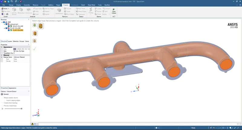
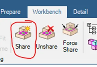
Then, we would check for interference and repair it if any is present. Now in order to get the conformal mesh ensuring perfect contact between the meshes, we enable the "Share topology" option, and then in "Workbench" enable the "Share" option.

Y+ Selection and Validation:

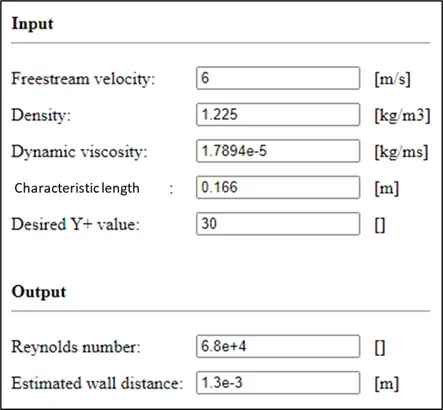
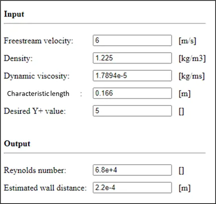
The Y+ selection for this case was made in 2 stages. 1st stage was with the idea of the nature of the flow, wherein since the flow is turbulent in nature we chose the Y+ value as 30 and the second stage was since we need to calculate the near wall effects(Convective Heat transfer Coefficient), we go with the lower Y+ value of 5.

Eventually, after simulating a trial run, we can find out the real Y+ value using fluent. From the XY Plots, when we plot the Y+ function under the turbulence section, we will get the Y+ values highlighted.

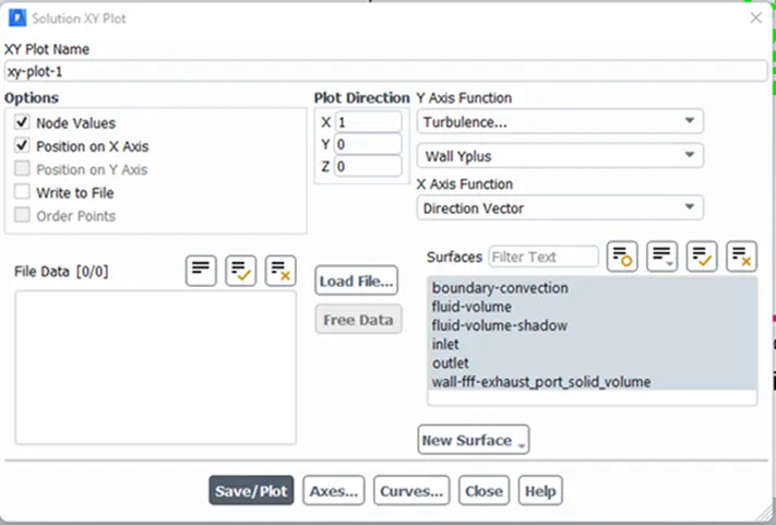
If the selected Y+ value was correct then the plot also indicates the same value.

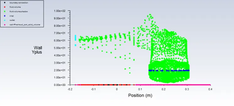
Here for the above plot, the selected Y+ value was 30, but it indicates some lesser value. Thus this is not the accurate prediction made for the Y+ value.

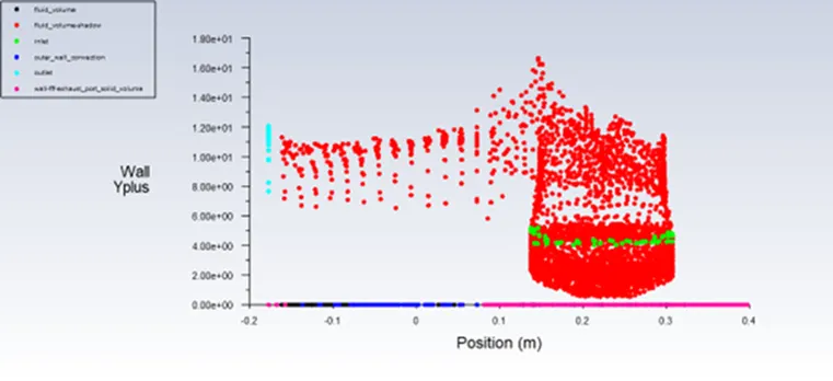
Here the plot matches the value of Y+ precisely as 5. Thus, our predicted Y+ value of 5 is accurate for this study case.

Meshing:

First of all, the named selections are imparted. There are 4 named selections given and they are.

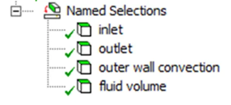
The inlet is applied to all 4 pipes and the outlet to the converging one. The outer wall convection is for the solid volume and the fluid volume as a separate naming.

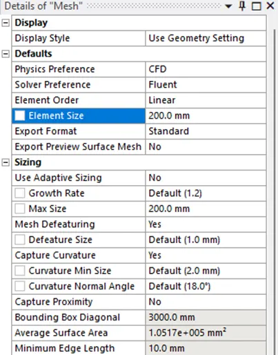
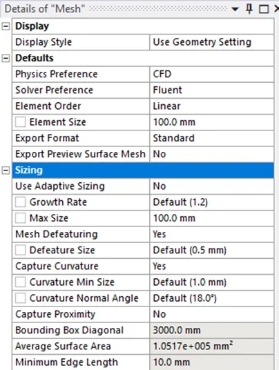
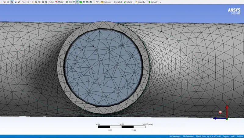
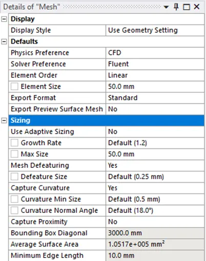
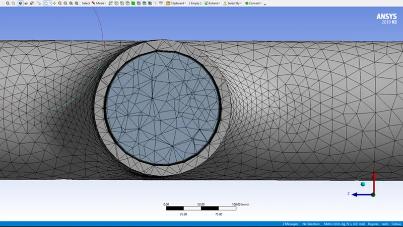
The meshing was done for 3 different cell sizes, wherein both the outer wall and fluid volume are given the same size. The sizes are, 200mm, 100mm, and 50mm.

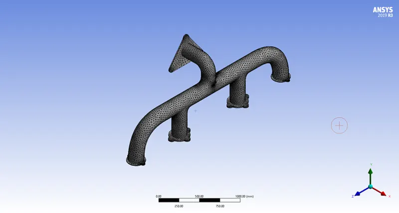
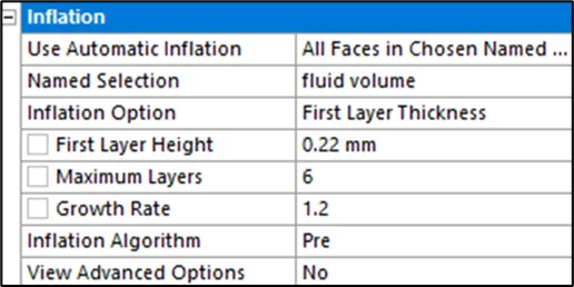
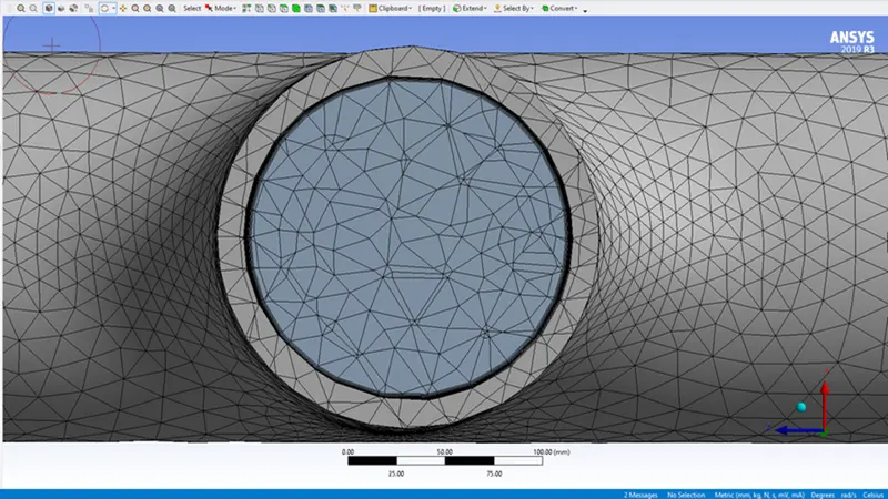
The inflation layers were developed for the fluid volume from the previously discussed Y+ value optimization. The total number of inflation layers is 6 and the first layer thickness is 0.26mm for the Y+ value of 5.

1. 200mm:
   
2. 100mm:
   
3. 50mm:
   

Setup & Selection of Viscous Model:

The setup is done by initially turning on the “Energy equation” since it involves the temperature. Here we don’t need to set up the reference values since they are only applicable to external flow conditions. Now the next important step is to select the viscous model.

There are 2 viscous models which we can apply here. One is K-Omega SST and the other is Standard K-Epsilon models respectfully. Here one of our primary goals is to find the Convective heat transfer coefficient from the hot fluid to the solid medium. Thus, getting the precise properties near the wall is very important, for which better results are always given by the K-Omega SST model. Anyways we compare both models and observe the variations between those models.

The next step is to set up the boundary conditions wherein the inlet velocity is mentioned as 6m/s as discussed above from the velocity calculations and the inlet temperature is given as 650K(376.85^oC). The outlet B.C is set to zero-gauge pressure(atm). For the outer wall, the convective heat transfer coefficient the HTC value was given as 20 W/m²K (of air) which is the value obtained from the study.

Then we initialize the solution with the hybrid model. And then we run the simulation for nearly 150 iterations.

Analytical Solution for finding the approximate value of HTC from the fluid to solid:

The HTC for a flat plate is calculated and the values for the internal flow can be related to it since it differs only slightly.

Velocity=6m/s

Reynolds Number(Re)= (Density x Velocity x Charact Length) / (Dynamic Viscosity)

= (1.225 x 6 x 0.166)/(1.7894 x 10e-5) = 68185

Clearly, it is evident that the flow is turbulent in nature.

Prandtl number(Pr) for air @ 20^oC= 0.744

Nusselt number(Nu) = 0.664 x (Re)e0.5 x (Pr)e0.33= 157.27

Heat Transfer Coefficient(HTC)= (Nu x Thermal Conductivity) / Charac. Length = 23W/m²K

Therefore the HTC for our setup case must almost be equal to 23W/m²K.

Results:

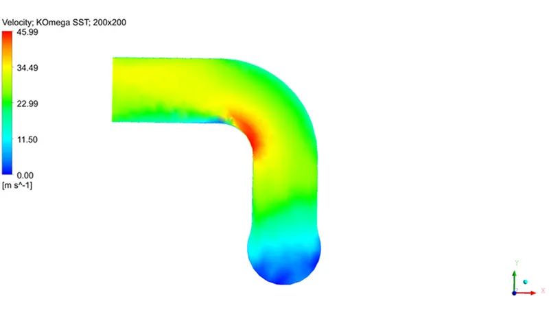
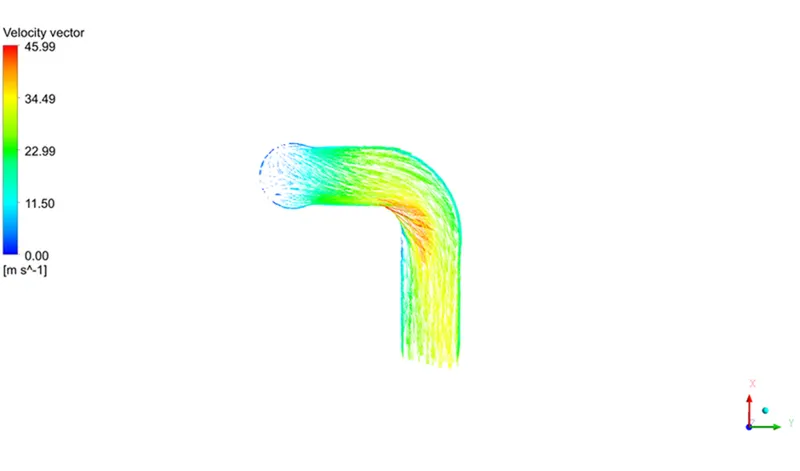
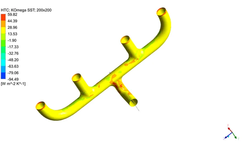
The Velocity and vector field in the central plane of the exhaust system and the Convective Heat transfer coefficient (HCT) contour around the boundary line of fluid and solid are examined.

Since it is an internal flow that involves continuous flow iterations can be limited to 150 which will itself lead to the best fit of the results. Iterations to 800 also will give the same results as 150 iterations.

The residual plot of the K-Omega SST viscous model and Standard K-Epsilon model are shown below.

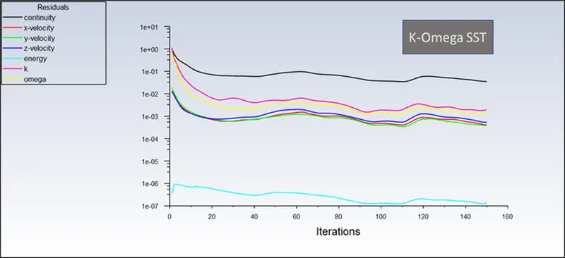
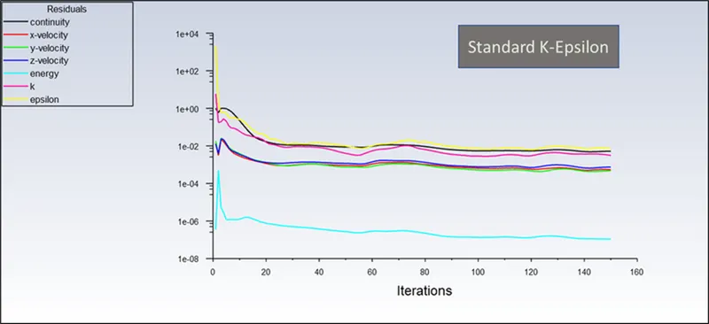
The above two figures are the general residual plots for almost all the considered mesh categories.

Also, the average HTC from the Fluent tool is calculated as directed below.

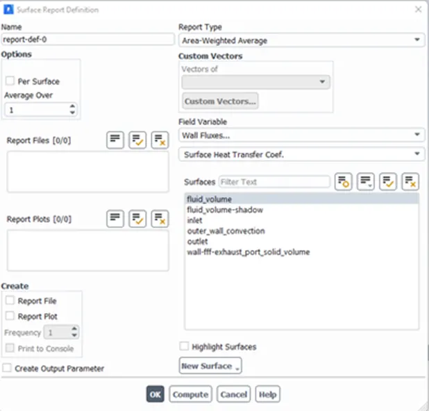
The Temperature contour in general will look as depicted in the picture below for almost both the viscous models respectively, with different mesh sizes.

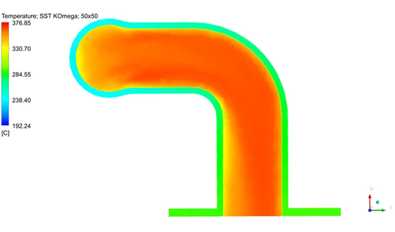
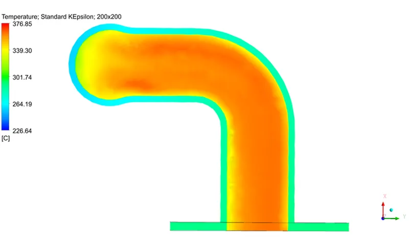
The only notable parameters are velocity and HTC.

Firstly, the comparison is made between both viscous models of the same size categories.

(i). 200mm:

K-Omega SST (200mm):

The results from the CFD Post are as follows,

Velocity Profile:

Vector Plot:

HTC Contour:

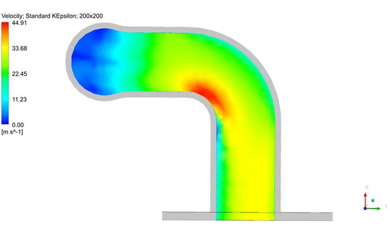
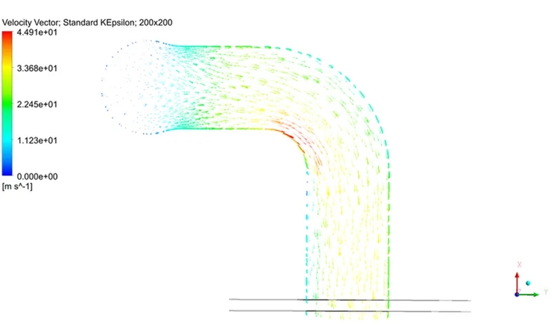
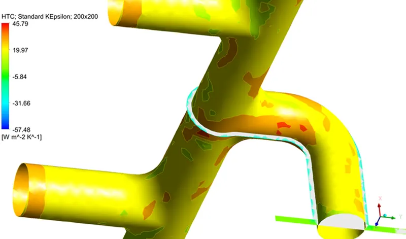
K-Epsilon Standard(200mm):

Velocity Profile:

Vector Plot:

HTC Contour:

Inference(200mm):

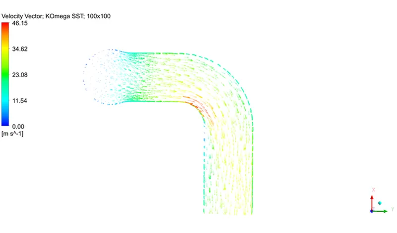
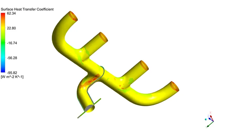
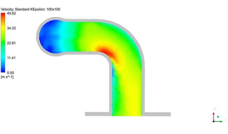
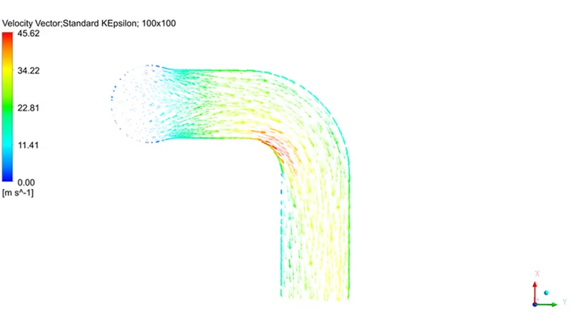
As discussed earlier, the K-Omega SST model captures the near-wall effects more precisely and the same has happened here in the case of the Heat Transfer Coefficient (HTC). In this case, since it is a converging tube, as per the mass flow rate equation, the velocity at the outlet will be high compared to the inlet and highest at the bend of the converged tube. Thus, Heat transfer takes place more at the region where velocity is more (K-Omega SST: 46 m/s; K-Epsilon Std: 44.91 m/s). The maximum HTC captured by the K-Epsilon model (45.79 W/m²K) at that bend region is lesser than what is gained from the K-Omega model (59.82 W/m²K). However, the average HTC sums up to 21.5 W/m²K for both models. Anyways we will give it another try with further mesh refinement.

(ii). 100mm:

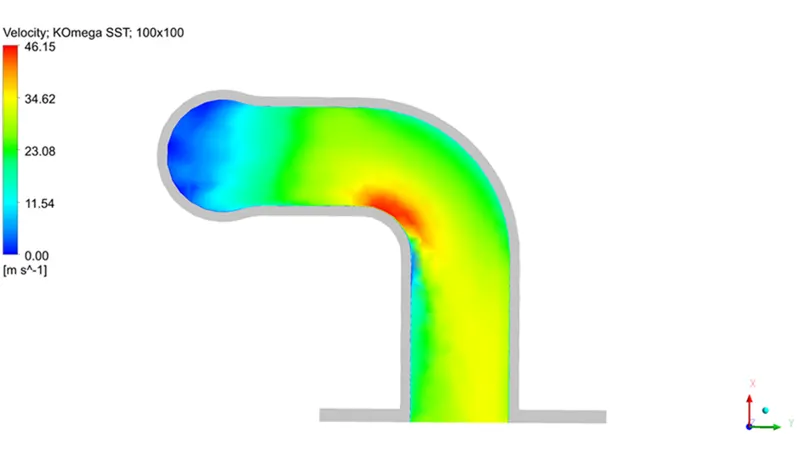
K-Omega SST (100mm):

Velocity Profile:

Vector Plot:

HTC Contour:

K-Epsilon Standard(100mm):

Velocity Profile:

Vector Plot:

HTC Contour:

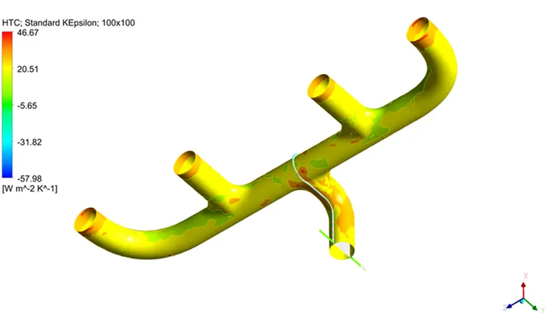
Inference(100mm):

The same inference which we have said for the 200mm mesh size is applicable here too. The maximum HTC captured by the K-Epsilon model (46.67 W/m²K) at that bend region is lesser than what is gained from the K-Omega model (62.34 W/m²K). However, the average HTC sums up to 21.5 W/m²K for both models. Hence, we now move ahead with the refinement process considering only the K-Omega SST viscous model. The maximum velocities at the bent section are (K-Omega SST: 46.15 m/s; K-Epsilon Std: 45.62 m/s).

(iii). 50mm:

K-Omega SST (50mm):

Velocity Profile:

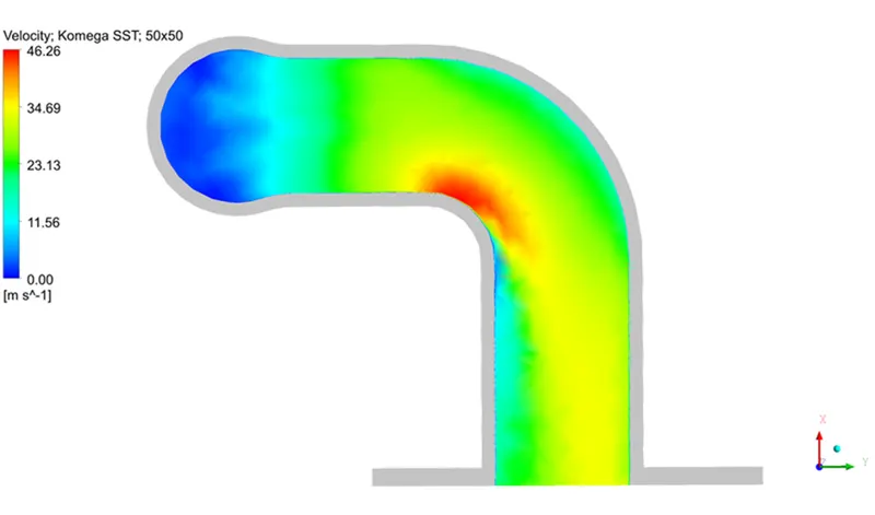
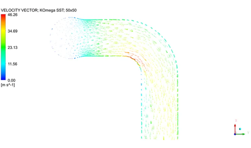
Vector Plot:

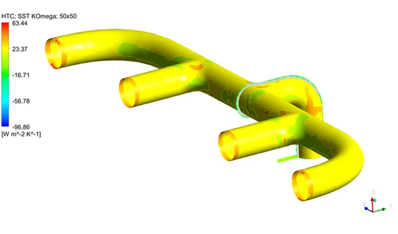
HTC Contour:

Inference(50mm):

Here the maximum HTC value is about 63.44 W/m²K and it also gives the maximum HTC values of the considered mesh sizes. The maximum velocity at the bent section is 46.26 m/s.

The conclusion from the comparative study:

The below table comprises the grid independency test results, from which certain points are made as conclusions.

S.No	Mesh size(mm)	Viscous Model	Max HCT (W/m2K)	Avg HCT (W/m2K)	Max Velocity (m/s)	Cell count
1	200	Standard K -Epsilon	44.91	21.532	45.79	275513
		K-Omega SST	59.82	21.29	46
2	100	Standard K -Epsilon	46.67	21.44	45.62	275203
		K-Omega SST	62.34	21.15	46.15
3	50	K-Omega SST	63.44	21.15	46.26	275587

From the study, it is observed that the average HTC value is almost equal to the analytical value calculated for the freestream flow over the plate(23 W/m²K) and is almost the same for both models with different mesh sizes, but the maximum HTC value differs. As the mesh is refined, it precisely captures the maximum HTC value, and hence the mesh size of 50mm shows the best result. Since the cell count is not that different for the most refined case of 50mm mesh size but yields the best result, it can be chosen as an effective mesh size.

Source:

1. Conjugate Heat Transfer - CONVERGE CFD Software
2. CFD Online - Y-Plus Wall Distance Estimation (cfd-online.com)