Week 4 - CHT Analysis on Exhaust port

Aim = CHT Analysis on Exhaust port

Introductions (Theory of topic)

Where CHT analysis is used

conjugate heat transfer (CHT) analysis can accurately predict heat transfer by simultaneous solving all the relevant solid and flow field heat transfer processes, for example: conduction through solids, free and forced convection in the gases/fluids and thermal radiation.

The CHT approach has an advantage over FE thermal analyses in that wall heat transfer coefficients and their local variations on surfaces are directly calculated within the model rather than based on simplified empirical calculations. The CHT approach therefore has benefits for those applications where heat transfer is either non-uniform or difficult to calculate empirically.

why analysis is used

CHT analysis is required to control the cooling rate by predicting the heat transfer coefficient and to show the temperature variation of solid. CHT is also used in analyzing the heat transfer in a heat exchanger. A heat exchanger is a system where heat is transferred between two fluids (may be of different phases) without mixing of these two fluids. A Shell and tube heat exchanger is a perfect example of CHT, here one fluid flows through tubes and other fluid flows in the shell over the tubes. The heat is transferred from one fluid to the walls of the tube and then from the tube wall to other fluid. Here CHT analysis is useful for predicting the heat transfer coefficient and to improve the effective heat transfer rate. CHT is also used in analyzing the cooling of electronic devices.

importance in practical applications.

The analysis type Conjugate heat transfer (CHT) allows the simulation of the heat transfer between Solid and Fluid domains by exchanging thermal energy at the interfaces between them. In solids, conduction often dominates whereas, in fluids, convection usually dominates Conjugate heat transfer is observed in many situations. For example, heat sinks are optimized to combine heat transfer by conduction in the heat sink with the convection in the surrounding fluid. Other examples include simulation of heat exchangers, and general-purpose cooling and heart

The outcome of CHT Analysis:

The outcome of CHT Analysis:

• Temperature distribution analysis.
• Heat flux rate analysis - calculation of wall heat flux rates or heat transfer coefficients.
• Visualization of heat transfer features for improved understanding of system flow phenomena
• Identification of localized 'hot spots or heat sinks in checking against specified requirements
• Evaluating variation in temperature peaks for different operating conditions/ failure modes
• Assessing insulation or heat shield effectiveness and optimizing of material selections Coupling CHT with FE analysis to evaluate thermally induced stresses, expansion or fatigue.

Maintain the y+ value according to the turbulence model and justify the results

Value of y+ is taken in range of 0<y+<05. So we have to take k omega model because we want surface wall heat transfer coefficient and as we know k omega is used for solving equation for near the wall of boundary

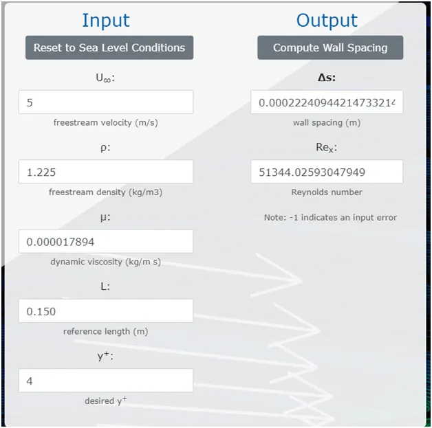
As we saw in output wall spacing value is 0.00022m but this is the distance from centre to boundary of wall or boundary of first inflation layer of mesh. So height of 1^st first inflation layer is two times of 0.00022m which is equal to 0.00044m and 0.44mm.

It is divided in 5 parts

• Geometry
• Mesh
• Setup
• Solution
• Result

Geometry section

Here we have to creat a model of exhoust port in spaceclaim of workbench.

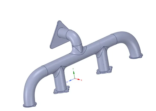
model of exhoust port

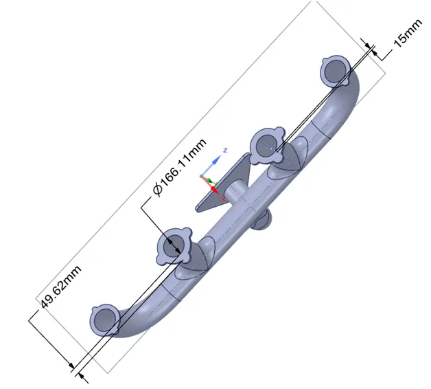
For anlysis of conjugate heat transfer (CHT) on exhoust port we have to fill fluide in the exhaust pipe.

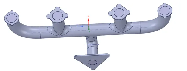
After filling the fluide materia in hollow pipe we use share option in workbench.

When we use share option the mesh boundary of two bodys (solid mesh and fliude mesh) are perfectly interfacing there adges with each other. It means there is no any physical distance in between two meshes.

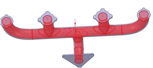
After hit the share option from workbench then this red coloured boundary is show where the faces of meshing boundary of two body are interfacing with eachothere. And surface boundary of two face are become pink colour it means share option is apply perfectly.

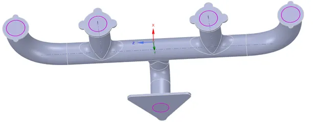
good interfacing mesh.

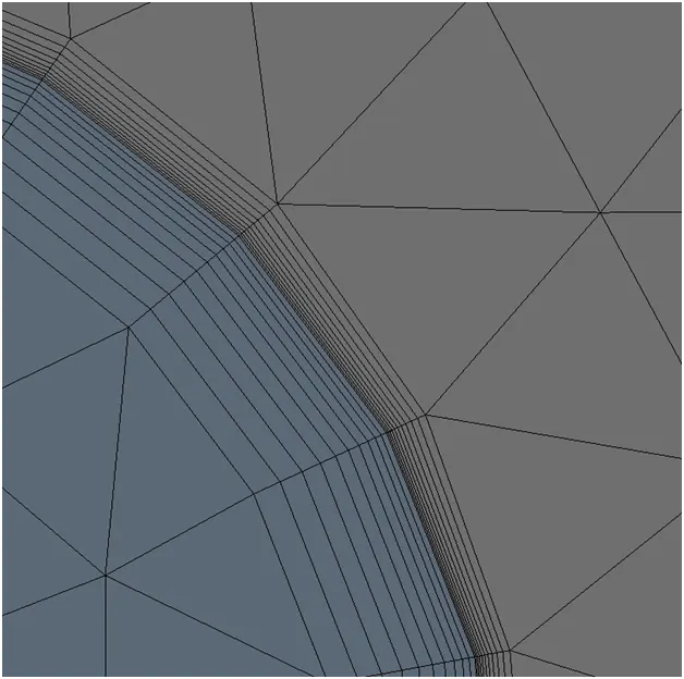
After applying share option meshing look like this as shown in above figure. and here geometry section is complete and close it.

Meshing section

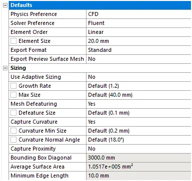
When we open mesh section then all data which is generated in geometry part is automatically transfer in mesh part and geometry is ready for mesh. Here we have to put mesh element size is 20mm in mesh setting and then generate the mesh.

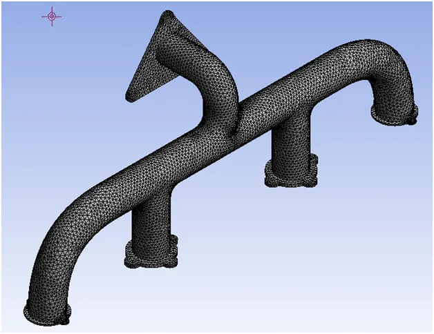
Back side view

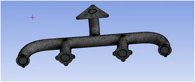
Front side view

After creating mesh we have to apply inflation layer at solid and fluid boundary.

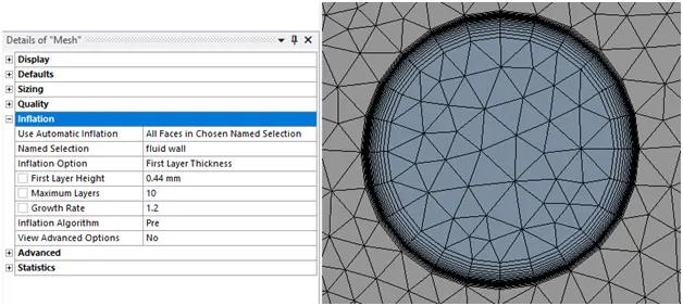
Here we use first layer thickness method because we know the thickness of first layer which is 0.44mm which is calculated by y+ calculator.

Thickness of first layer 0.22*2=0.44mm

After creating inflation layer then check the number of element and number of nodes in the whole mesh.

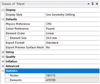
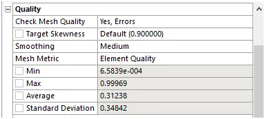
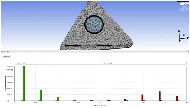
As we see here total number of element is 470709 which is nearly 0.5 million so this is enough number of element in this geometry.And finally check the meshing quality.

Naming the all section of exhaust pipe.

Inlet

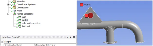
Outlet

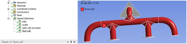
Fluid wall

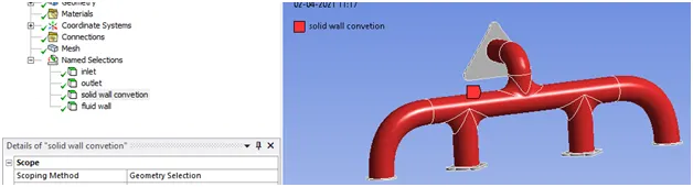
Solid wall

Setup section

Here we have to setup condition or provide input for simulation to the geometry. When we open the setup section then the geometry structures is appear automatically and green arrow indicate inlet port and red arrow indicate outlet port.

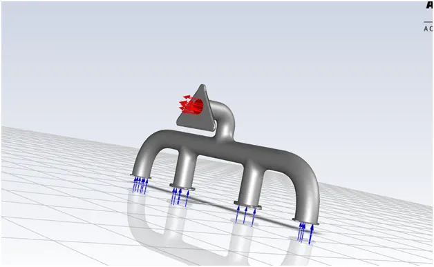
General setup

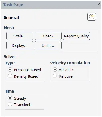
Here we use pressure based solver, absolute velocity, and steady state condition. These are the general condition.

Energy equation

Here in simulation we play with variation of temperature and velocity in the exhaust pipe and fluid that’s why we use energy equation.

And for viscous model.

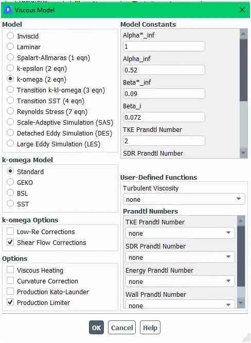
Here we use standard k omega model because our Reynolds number is lie in between 0 < Re < 05 and we know that velocity near the boundary is very small that’s why value of Reynolds number is very small.

Materials which is used in exhaust pipe

Fluid material

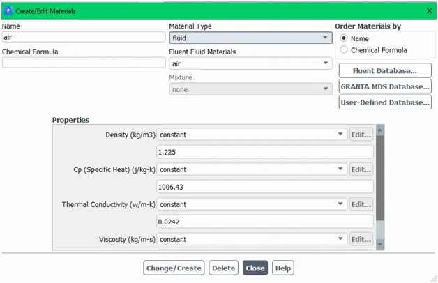
Here we use air as a fluid material

Solid material

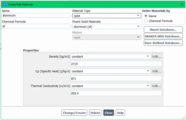
Here we use aluminium as a solid material.

Boundary condition

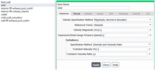
Inlet conditions here inlet velocity is 5m/s.

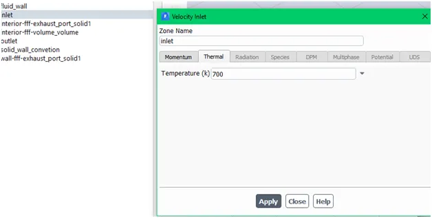
Inlet thermal condition is 700 k.

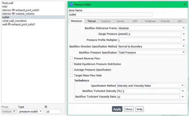
Outlet condition where gauge pressure is 0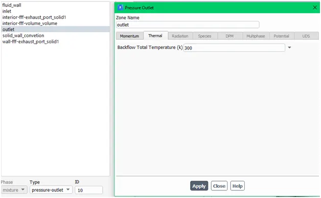

Thermal condition at outlet is 300 k.

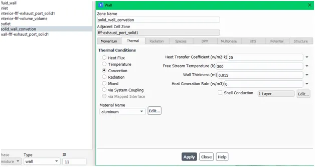
Here we use convection on the solid wall and heat transfer coefficient is 20(w/m2-k).

After setup the conditions then we have to create contour of velocity and temperature variation so we have to initialize first.

And then create contour at solid wall convection.

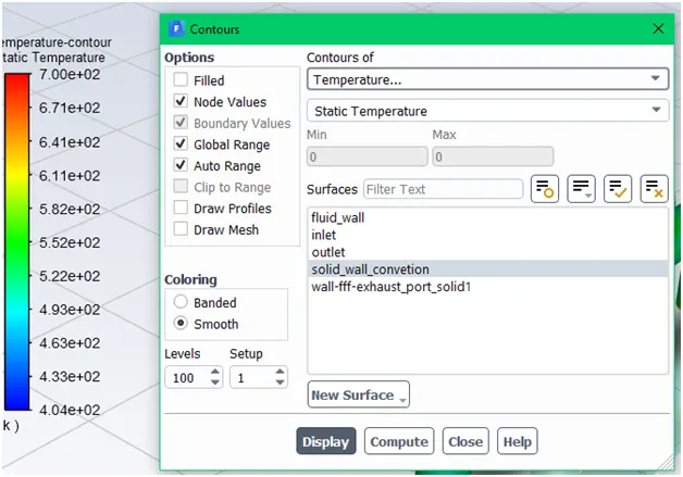
After creating contour create animation of temperature of solid wall convection and hit the calculate option for 150 iteration. After complete the 150 iteration we get result in animation form.

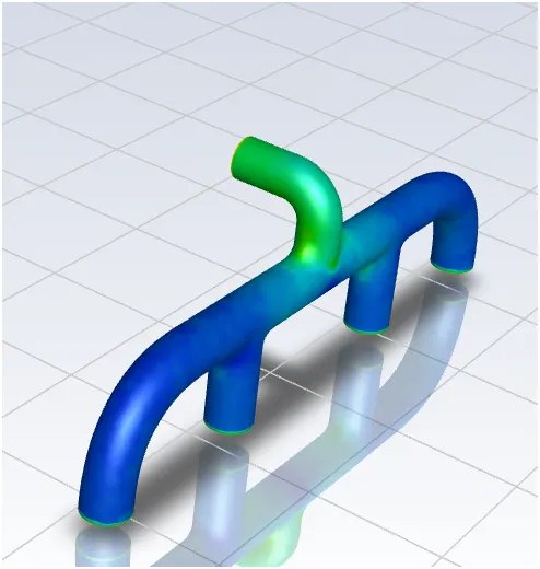
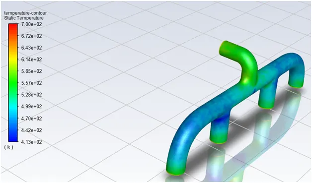
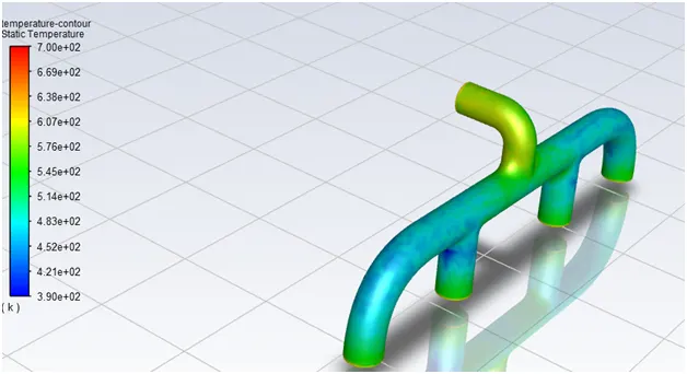
As we seen in above figure the temperature of every place on solid surface is getting vary.

Result section

In result section we can justifying the simulation and the result which produce in solution section. For verifying our result we can use different tools which is available in result section

Stream line Velocity

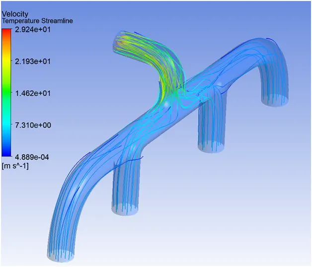
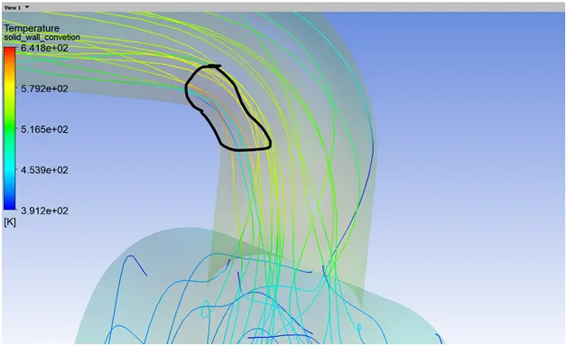
As we saw the stream line near the wall in bending part of exhaust pipe is red in colour it means the temperature near at the bending part is more as compare to other part.

Temperature on the solid wall.

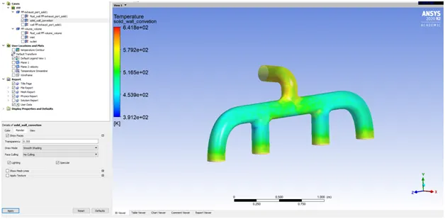
In above figure show temperature is vary with location on solid wall.

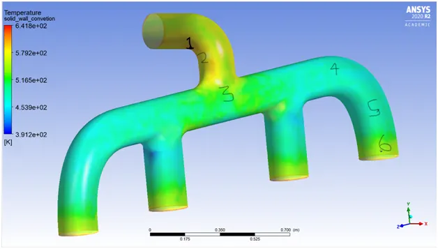
Here at point 1 have 613.726 k

Point 2 594.586 k

Point 3 562.586 k

Point 4 542.665 k

Point 5 498.255 k

Point 6 552.566 k

By analysing the data we can say that most heated part of the exhaust pipe is bending part of outlet pipe.

If steady flow exists in a channel and the principle of conservation of mass is applied to the system, there exists a continuity of flow, defined as: "The mean velocities at all cross sections having equal areas are then equal, and if the areas are not equal, the velocities are inversely proportional to the areas of the respective cross sections." Thus if the flow is constant in a reach of channel the product of the area and velocity will be the same for any two cross sections within that reach.

Where:

Q = the volumetric flow rate

A = the cross sectional area of flow

V = the mean velocity

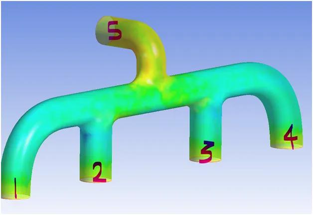
Q=A1V1+A2V2+A3V3+A4V4=A5V5

By continuity equation we can say that velocity at outlet is much more as compare to inlet. So when velocity is getting increase then Reynolds number is also increase and then rate of heat transfer is also increase.

And as we discussed above velocity near the boundary at bending section at outlet is more so the heat transfer rate at that place is also getting increase.

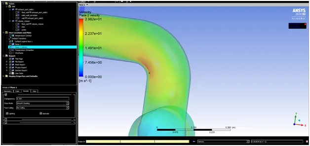
As we discuss above at this part have more velocity and also temperature.

Wall heat transfer coefficients.

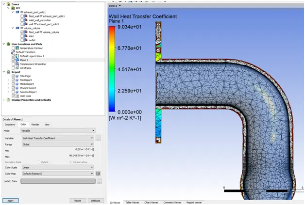
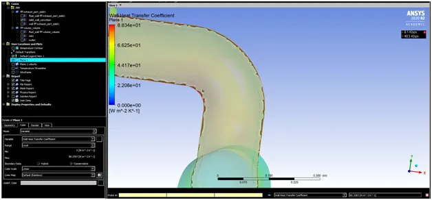
Max wall heat transfer coefficient at this place is 80.3282wm^2k^-1

Temperature of fluid wall

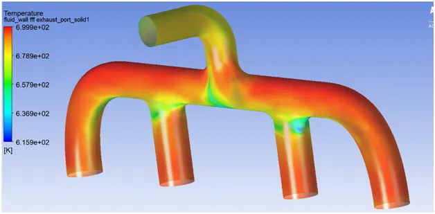
As we saw in above figure temperature at inlet wall is more but at inlet temperature is (300k) and temperature at outlet wall is less but temperature at outlet wall is (700k) this is because rate of heat transfer.

At inlet the velocity of hot gas is less so rate of heat transfer is also less and heat is trap in the pipe but at outlet velocity of gas is more so rate of heat transfer is also more and heat is not get trapped in the outlet wall.

Conclusion

In this study CHT analysis has done to find out temperature rise manifold because of hot air passing through it and we predicted heat transfer coefficient as well Velocity contours were created to get insights of fluid path and maximum velocity area.

It can be seen that heat transfer coefficient is more near the wall where the wall or exhaust pipe is bend.