Steady Vs Unsteady flow over a cylinder

Aim :-Steady and transient flow simulation of flow over cylinder, explain the phenomenon of vertex street

Geometry preperation

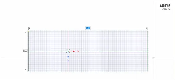
In this project simulation is done on the two dimensional geometry which is constructed below

Procedure

• Open workbench and drag the fluide flow (fluent) right side, then open 1^st option geometry.
• Then before we move further we have to change unit of length by clicking spaceclaim option in file.
• In spsce claim select circle from design, draw a circle of diameter 2M, chose condtrution line and construct 20M inlet line and 40M outlet line from the centre of the circle.
• 10M above and 10M below the centre of circle of symmetry.
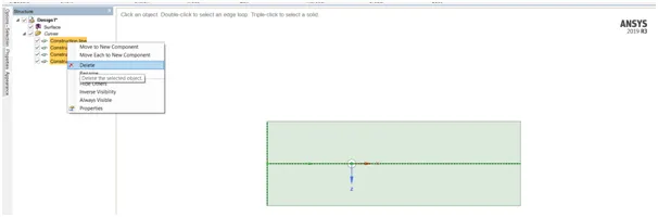
• After clicking on pull select the geometry then go again and select the circle and then press the delete option.

Meshing

• First naming the wall,inlet,outlet and symmery of the wall of the cylinder.
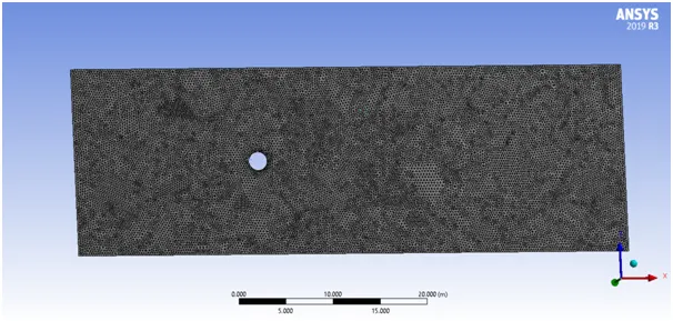
• Select the mess size and put it 0.25m after right click on mess choose select method in insert.
• In automatic method select the geometry and in method choose tringle.
• Again right click on mess select sizing in sizing select adge in type chose number of division put .
• Right click on mess in insert select inflation,geometry select face,boundry select cylindrical sdge,infletion option select first layer thickness,first layer height put 5e-3,maximum layer 6 there after right click and apply generate mesh.

Kármán vortex street

In fluid dynamics, a Kármán vortex street (or a von Kármán vortex street) is a repeating pattern of swirling vortices, caused by a process known as vortex shedding, which is responsible for the unsteady separation of flow of a fluid around blunt bodies It is named after the engineer and fluid dynamicist Theodore von Kármán,^[1] and is responsible for such phenomena as the "singing" of suspended telephone or power lines and the vibration of a car antenna at certain speeds.

setup

property of fluid

density= 1kg/m^3

viscosity= 0.02kg/m-s

initialization= hybrid

Initial velocity condition for each case is varying here we taken k-epsilon model. Monitor point as taken as 8m behind the cylinder to monitor the change in velocity in each iteration.

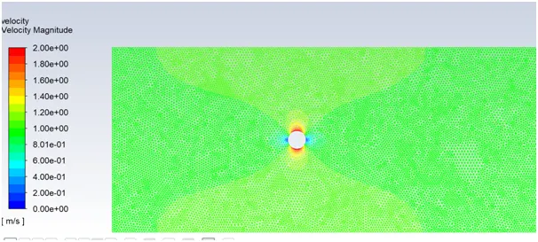
velocity contour at the time of initialization.

Part 1

Case (A)

Use steady state solver to simulate flow with Reynolds number= 100

Nu of iteration= 500

Inlet velocity= 1m/s

Case(B)

Use unsteady state solver to simulate flow with Reynolds number 100

Inlet velocity=1m/s

Time step=0.1

Number of time step=more than 1200

Compare the result of steady and transient(unsteady) state

Residual plots

Steady state unsteady state

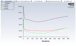
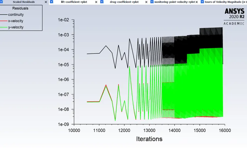
In case of steady state residual is not oscillating when iteration is increasing for transient state we observe the fluctuation is occur and it start to oscillation.

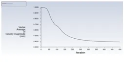
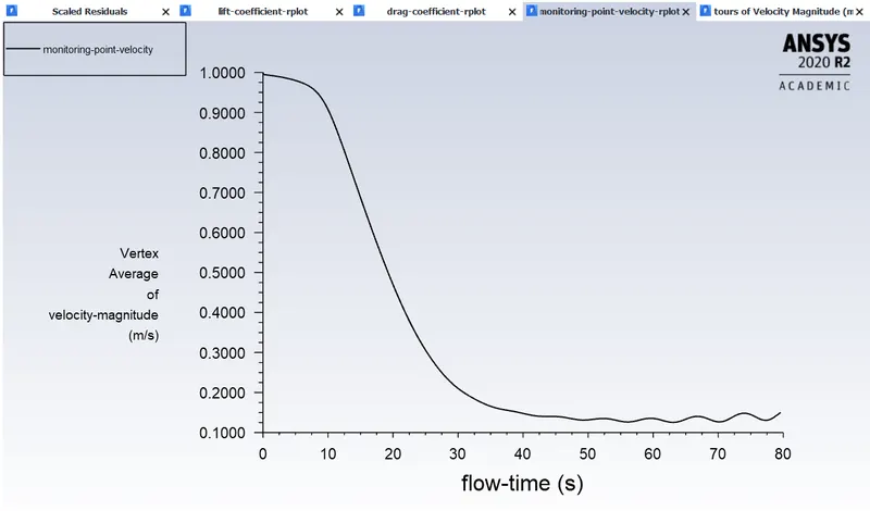
In steady state velocity with respect to iteration there is no fluctuation as we seen in figure but when we run for more than 1000 number of iteration then we show that it start fluctuate but in transient state it start fluctuate after 50 to 60 number if iteration.

Steady state unsteady state

steady unsteady

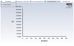
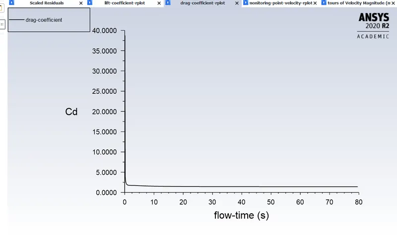
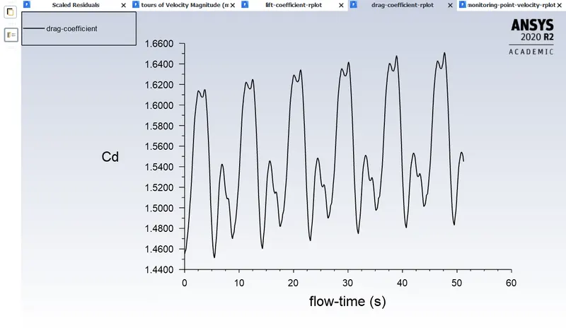
Coefficient of drag is constant for both in steady state and transient solver avg Cd for transient state solver is 1.4167.

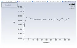
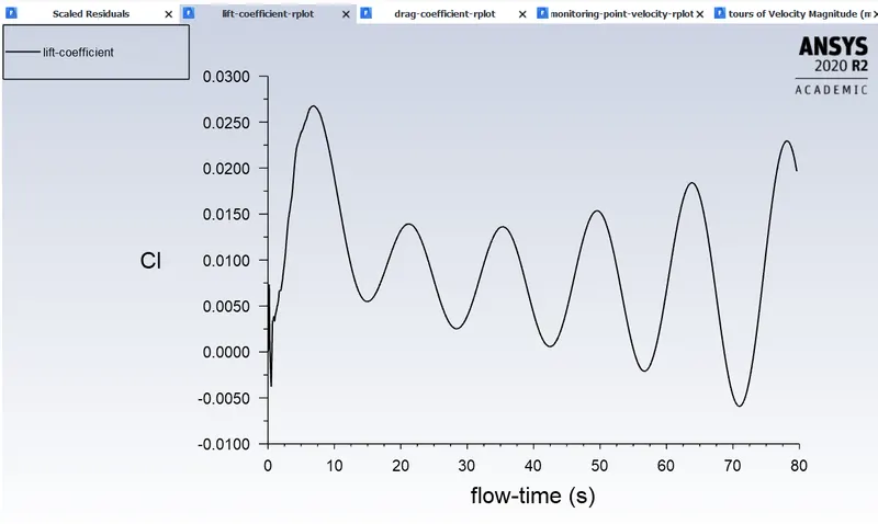
Coefficient of lift is slightly varying for steady state for transient solver fluctuation is more when iteration increases oscillation and frequency both increasing avg CI for steady state solver is 0.01452

steady unsteady

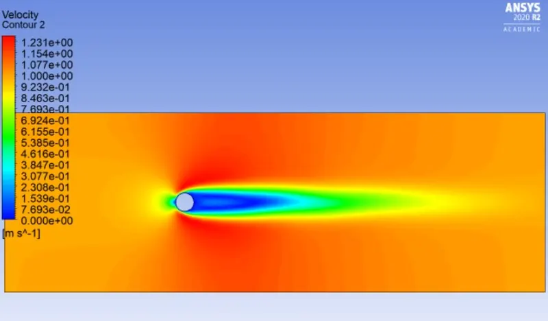
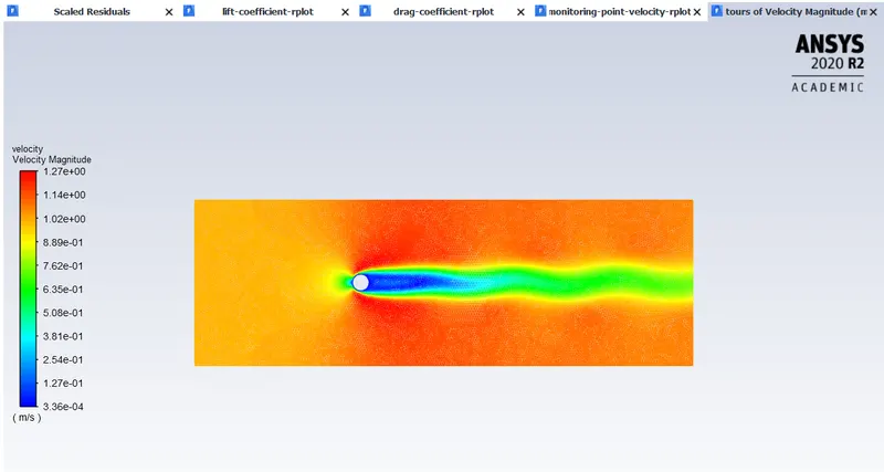
As we see in the figure in steady state it not fluctuate but in unsteady state as we see it start to oscillating after a certain number of iteration.

Calculation of strouhal number for transient state from monitor point velocity plot

The strouhal number is a dimensionless value useful for analyzing oscillation unsteady fluid flow dynamic problems.

The strouhal number can be expressed as

St= f*D/v

St = strouhal number

f=oscillation frequency

D=Diameter of cylinder

V= flow of velocity

The strouhal number are important when we realizing unsteady oscillating flow problem. The strouhal number represents a measure of ratio of the inertial force due to the unsteadiness of the flow or local acceleration to the inertia forces due to changes in velocity from one point to other in the flow field.

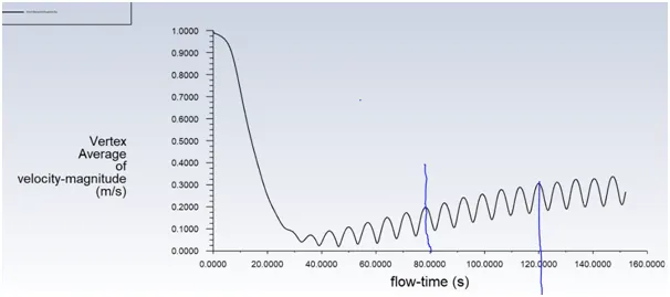
No of cycle = 6

Flow time =40s

Frequency(f) = no of cycle/flow time

=6/40

=0.150

St= f*D/v

=0.150*2/1

=0.30

Part-II

For unsteady state Reynolds number Re =10,100,1000,10000,100000

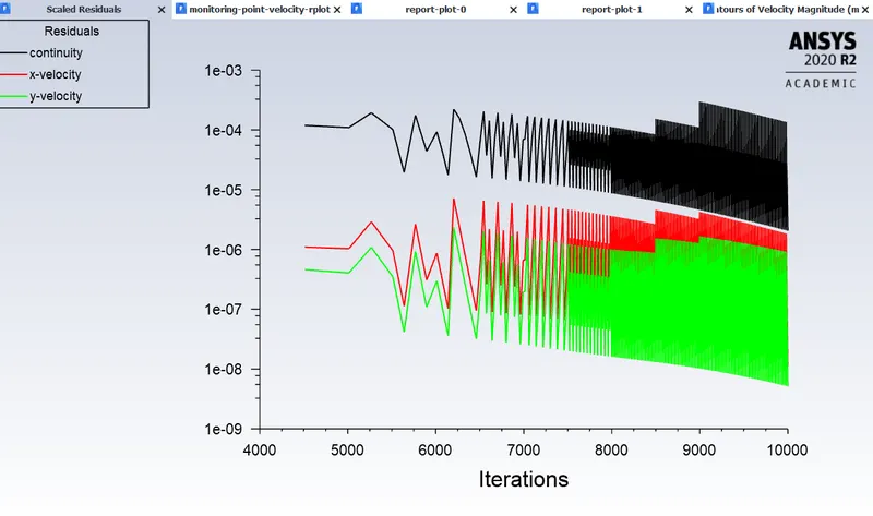
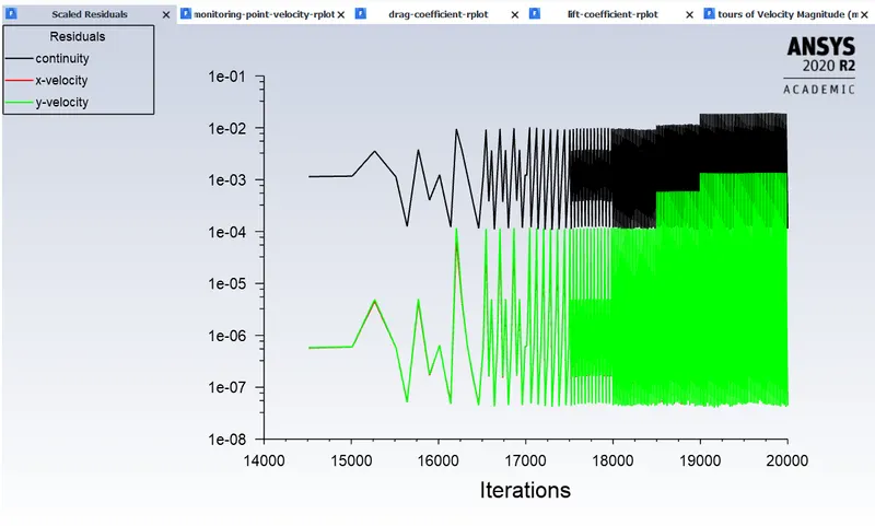
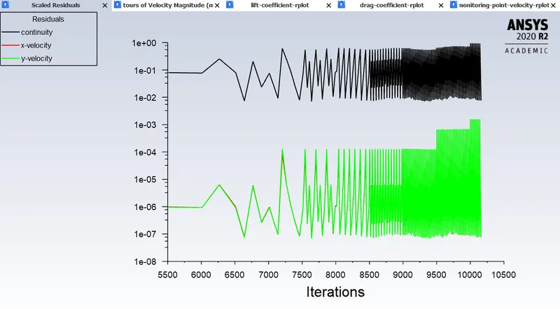
1) Residual plot for different Reynolds number.

Re=10 Re=100

Re=1000 Re=10000

Re=100000

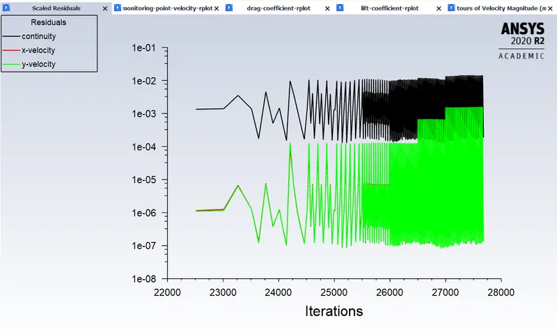
From the above resudal plot,we can say that when Reynolds number are increased rate of conversion or fluctuation is increased.

As we seen in above figure Re=10 fluctuation is start from around 6500 iteration

Re=100 fluctuation is start from around 12500 iteration

Re=1000 fluctuation is start from around 17000 iteration

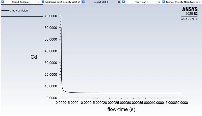
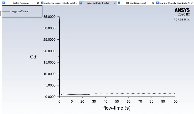
2) Coefficient of drag plot for different Reynolds number.

Re=10 Re=100

Re=1000 Re=10000

Re=100000

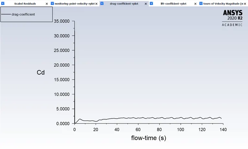
When Reynolds number is increased the drag coefficient is decreases.

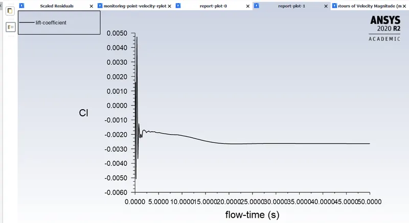
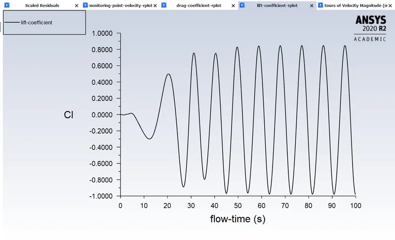
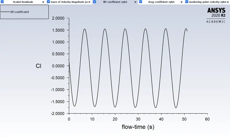
3) Coefficient of lift for different Reynolds number

Re=10 Re=100

Re=1000 Re=10000

Re=100000

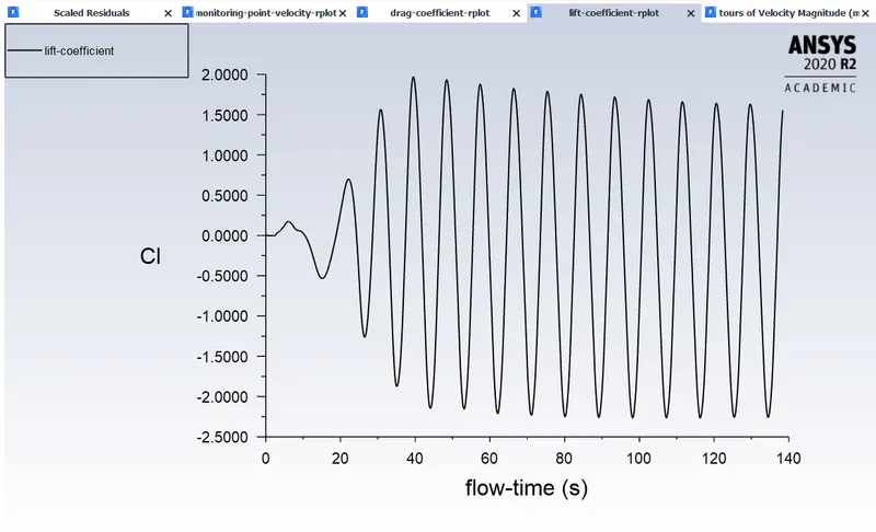
For low Reynolds number of lift is not fluctuate but when we increase the Reynolds number fluctuation of fluctuation is also increases.

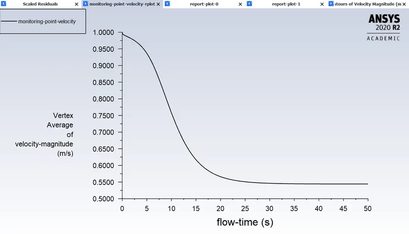
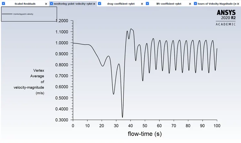
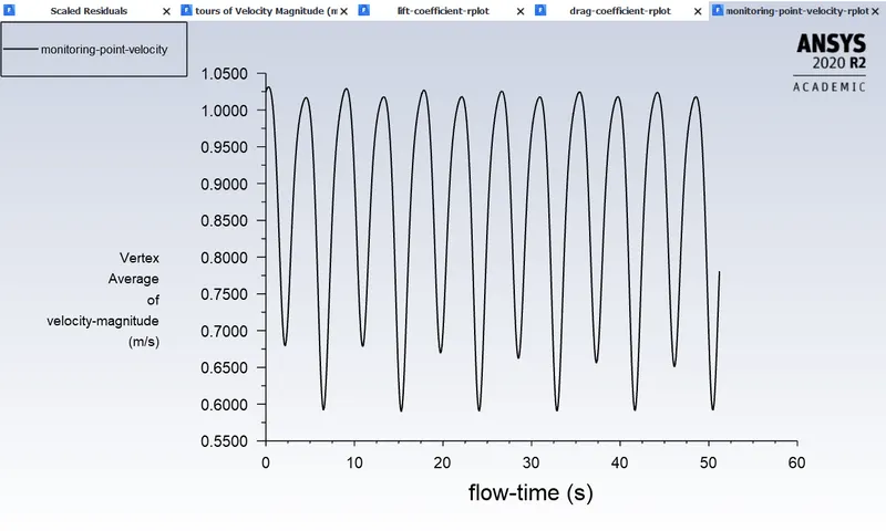
4) Velocity plot for different Reynolds number.

Re=10 Re=100

Re=1000 Re=10000

Re=100000

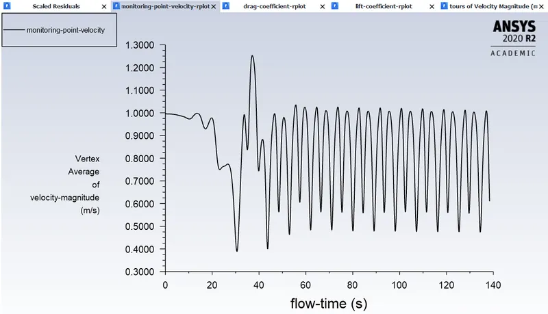
• From the plot of Reynolds number 10 when the number of iteration increases vortex seeding of monitoring point behind the cylinder was not experience.
• Further when we increases the Reynolds number at the same mess size (0.25), and same number of iteration vortex seeding of monitoring point behind the cylinder was experienced when Reynolds number are increases.
• Amplitude and frequency of the variation of velocity with respect to iteration increases when Reynolds number is increases.

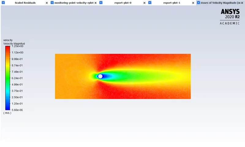
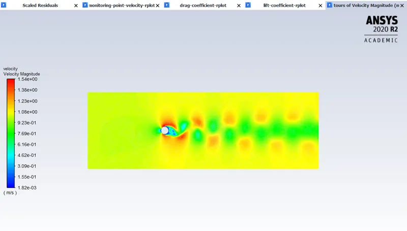
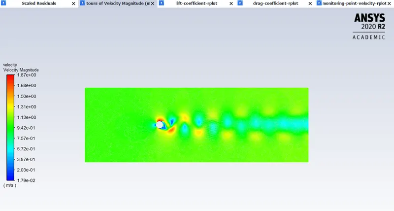
5) Velocity contour for different Reynolds number

Re=10 Re=100

Re=1000 Re=10000

Re=100000

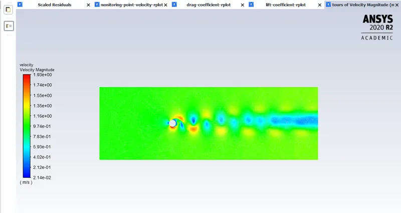
• For Reynolds number 10 vertex shedding was not showing there for velocity is constant behind the cylinder.

• For higher value of Reynolds number from 100 it start generating vertex shedding. Further increases the Reynolds number then frequency of vertex shedding is also increases.

6) Animations for different Reynolds number

Re=100

Re=1000

Re=10000

Re=100000

For higher value of Reynolds number from 100 it start generating vertex shedding. Further increases the Reynolds number then frequency of vertex shedding is also increases.

• Observation from the above plot

Reynolds number	Drag coefficient (avg)	Lift coefficient (avg)	Monitoring point velocity (avg)
Re=10	3.4015	0.00077	0.04614
Re=100	1.4167	0.01452	0.3901
Re=1000	0.73166	0.02644	5.0522
Re=10000	0.7039	0.2863	84.1745
Re=100000	0.41193	0.2721	762.79

Conclusion

• Vertex shedding was generate when Reynolds number is increasing from 100 Reynolds number.

• For higher value of Reynolds number coefficient of drag decreases is observed from the above plot and table.