Week 4 - CHT Analysis on Exhaust port

Aim:- Exhaust Port analysis.

Objective:-

1. Give a brief description of why and where a CHT analysis is used.
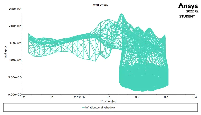
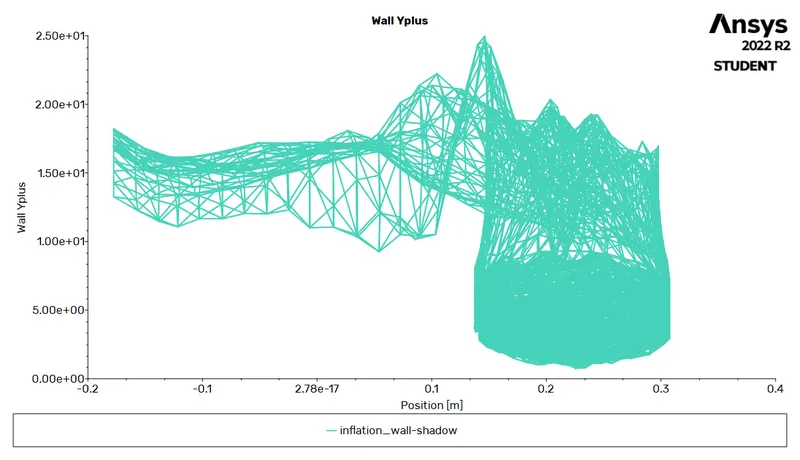
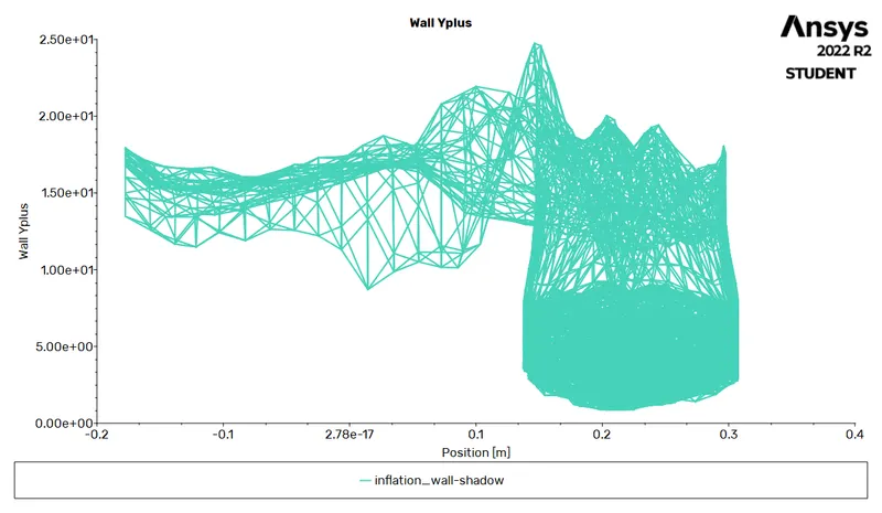
2. Maintain the y+ value according to the turbulence model and justify the results.
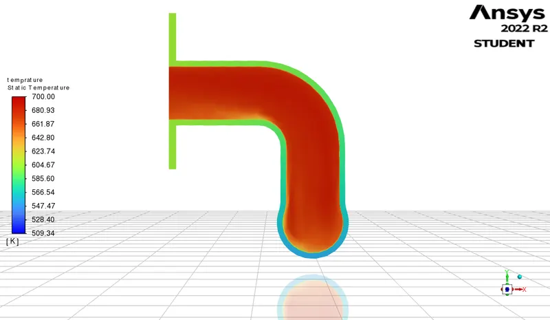
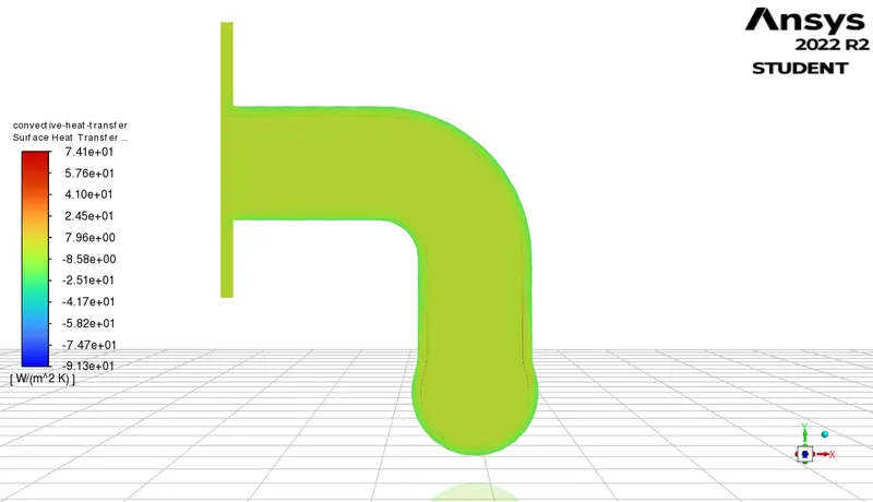
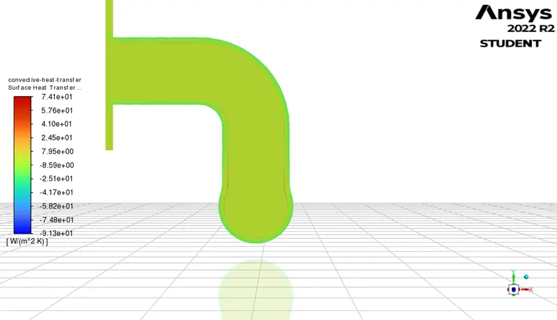
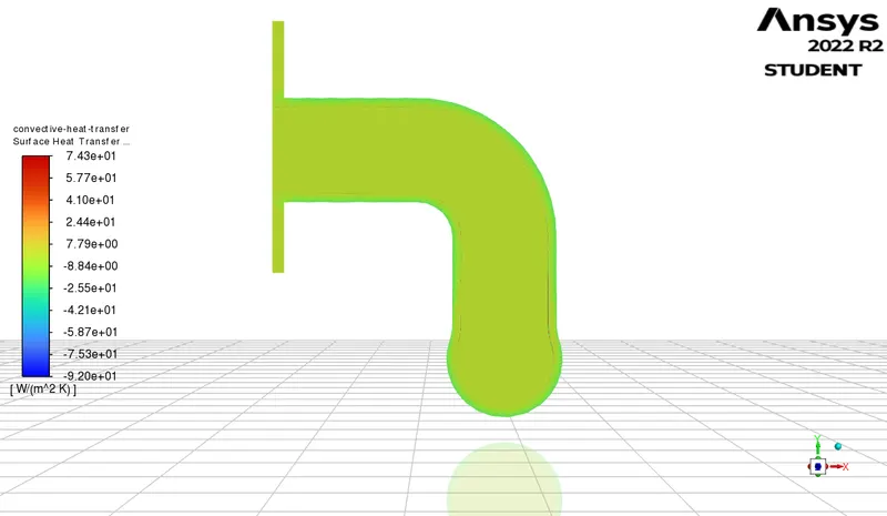
3. Calculate the wall/surface heat transfer coefficient on the internal solid surface & show the velocity & temperature contours in appropriate areas.
4. How would you verify if the HTC predictions from the simulations are right? On what factors does the accuracy of the prediction depend on?

Thoery: Fundamentals related with heat transfer.

Mode of heat transfer are

1. conuction

2. convection

3. radiation

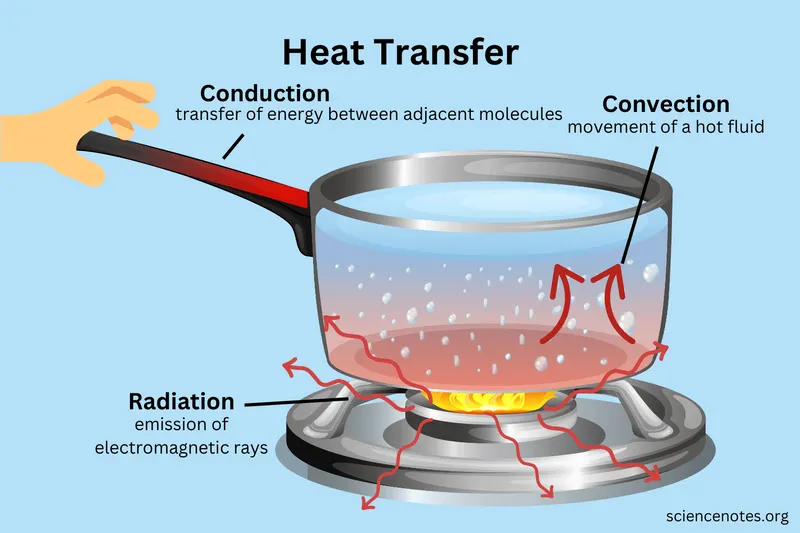
Conduction:- In conduction mode of het transfer the transfer is take place between adjacent molecules, bulk motion is not needed for heat transfer.

this can be calculated using fourier law.

for a plane layer, heat conduction layer for a plane layer is directly proportional to temprature difference and area across the layer but inversely proportional to the layer thickness

this can be governed by

Qc = -k A dt/dx

k is the thermal conductivity( unit Watt/m.k, it is a material property)

A is the area

dt is the temprature difference between the plane

dx is the thickness

Convection:- In convection mode of het transfer the transfer due to fluid flow, bulk motion is needed for heat transfer.

this can be calculated using newtons law.

heat convection directly proportional to temprature difference and area across

Qc = h A dt

h is the convective heat transfer( unit Watt/m^2.k)

A is the normal surface area

dt is the temprature difference between the plane

Radiation: Stefan Boltzman law of radiation

it state that radiation energy emitted from the surface of a black body is directly proportional to the 4th power of absolute temprature

Qr = sigma*T^4

sigma is stefan boltzman constant 5.67*10^-8 Watt/m^2k

Thermal diffusivity: is the ability of the material by which heat can propogate within the material

it is the ratio of thermal conductivity/Rho*c

here rho is the density (kg/m^3)

c is the specific heat (J/kg K)

Nusselt Number: Nusselt no is the ration of convective heat transfer to the conductive heat transfer

convective heat transfer/conductive heat transfer

hl/k

it is very important becuase it will tell which mode of heat transfer dominant, if nusselt no. is 1 then convective mode is dominating

Prandtle No.:- prandtle no. is the ratio of momentum diffusivity to the thermal diffusivity

miu(kinematic viscosity)/k(thermal conductivity)

Y+ model

The behaviour of the flow near the wall is a complicated phenomena and to distingish the different region near the wall the concept of wall has been formulated. This is the dimesnion less qunatity, and the distance from the wall measured in terrm of visous length

To resolve the effect near the wall i.e. inthe viscous sublayer then the size of the mesh should be small and dense enough near the wall so that almost all the effect can be captured

When any viscous flow flows over a surface, a region of slow-moving flow called boudary layer develops.

inside the boundary layer, there is a strong velocity gradient and u varies nonlinearly

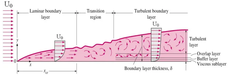
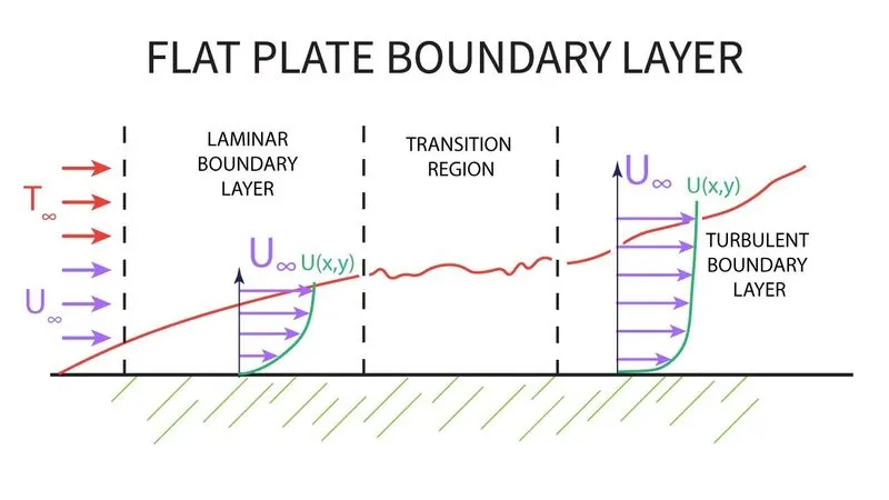
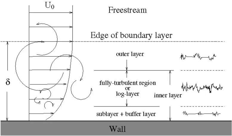
it is very important to distinguish between different layers to model the boundary physics correctly

For CFD SImulation we can compute the frist layer thickness values using online calculator

to calculate frist layer thickness we must have

1. free stream velocity

2. denisty of the fluid

3. dynamic viscosity

4. refrence length

5. refrence value for y+

Some refrence values for y+ are

for viscous layer .1 to 5

for buffer layer 5 to 30

for inertial sublayer 30 to 100

defect layer 1000 to 10000

for some models

for k-omega 1 to 10

for k-epsilon 30 to 100

for k-Omega sst 0 to 5

CFD:-Computational fluid dynamics or CFD is the analysis of systems involving fluid flow, heat transfer and associated phenomena such as chemical reactions by means of computer-based simulation.

Practical application in current scenario

• aerodynamics of aircraft and vehicles: lift and drag
  • hydrodynamics of ships
  • power plant: combustion in internal combustion engines and gas
  turbines
  • turbomachinery: flows inside rotating passages, diffusers etc.
  • electrical and electronic engineering: cooling of equipment including
  microcircuits
  • chemical process engineering: mixing and separation, polymer moulding
  • external and internal environment of buildings: wind loading and
  heating/ventilation
  • marine engineering: loads on off-shore structures
  • environmental engineering: distribution of pollutants and effluents
  • hydrology and oceanography: flows in rivers, estuaries, oceans
  • meteorology: weather prediction
  • biomedical engineering: blood flows through arteries and veins

CFD Work Flow:- CFD codes are structured around the numerical algorithms that can tackle fluid flow problems. In order to provide easy access to their solving power all commercial CFD packages include sophisticated user interfaces to input problem parameters and to examine the results

Its threee step process
(i) a pre-processor

involves defination of geometry, grid generation, selection of phenomenon that need to model

(ii) a solver

intergration of governing equation, discretisation and solution

(iii) a post-processor

ploting of contour, graphs and making movies.

In solving fluid flow problems we need to be aware that the underlyingphysics is complex and the results generated by a CFD code are at best asgood as the physics (and chemistry) embedded in it and at worst as good asits operator with CFD

Solving and Modeling Approch:-

There are no way present to understand and analyse the effeciveness of the mixiing tee model.

1. analytical approch

2. simulation approch

3. experimental approch

using analytical approch and experimental approch is time consuming and high cost senario. this could be eliminated by using simulation approch in which we can analyse the system with the actual codition we are intrested in.

To do this we are using ansys fluent solver

we are using fluid flow analysis using Fluent solver because we are interested in the total effectiveness of the fluid in the mechnical tee model, here we are using two different models to analyse the effectiveness of the mixing of fluid.

Approch we are using.

1. We need to open Ansys workbench

2. Choose the Appropiate Solver

3. Assign Appropiate name

4. Choose geometry and select new spaceclaim model.

5. Load the appropiate file

6. Implement the geometrical operation

7. Apply the mesh and provide name selection

8. Choose setup, select the appropiate model

9. Initalisation and running the simulation

10. Result making i.e. countour plots graphs

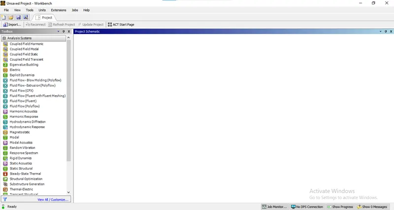
1. Opening Ansys workbench

2. Choose the Appropiate Solver

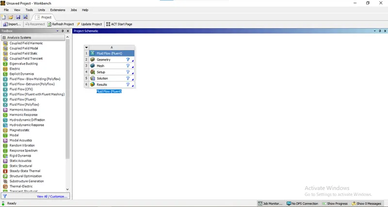
3. Assign Appropiate name:- Exhaust Port

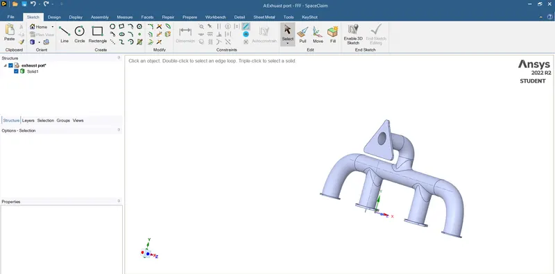
4. Choose geometry do to geometrical operation

choose the geometry>right click and choose space claim>choose the file

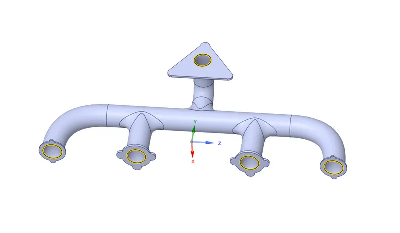
extrude the volume.

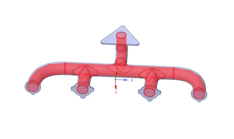
prepare>extract volume>choose the edge selection>select the edges>click ok> change names

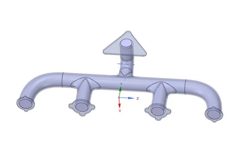
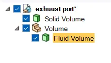
Now we need to use share the topology, just to ensure that connected body have shared faces

go to workbench>share>click ok

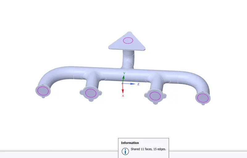
we done with geometry now we can move to mesh

Meshing

Now right click on mesh and choose generate option, it will create a mesh with defualt mesh legth of 150mm

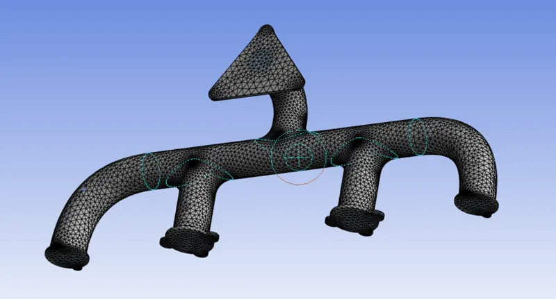
no we can provide name selection.

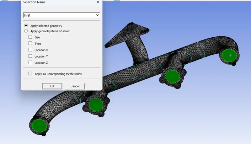
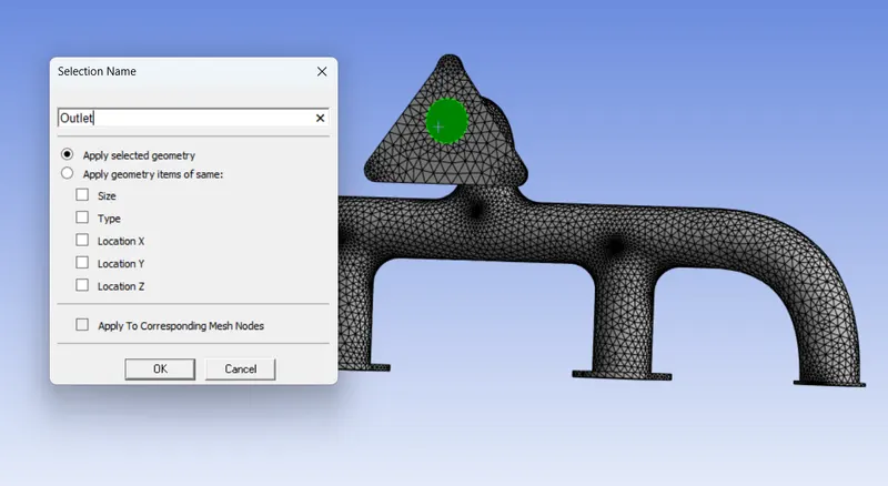
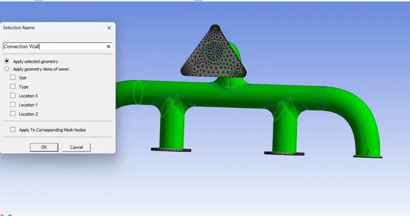
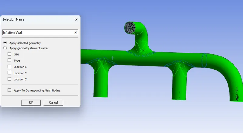
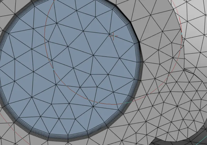
Now we provide inflation layer

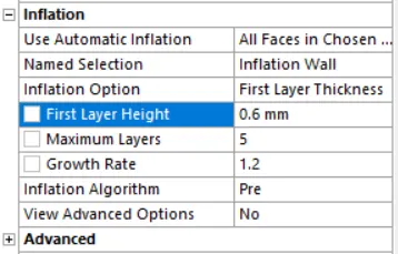
i calcuated the frist layer thickness from online y+ calculator with length as .166m an internal flow with velocity of 5 m/s

Setup

Settings

Solver	Steady State
Energy Equation	On
Model	K-omega sst
Inlet	Inlet Velocity 5m/s
Outlet	Pressure Outlet
Material_(Fluid)	Air(user defined)
Cell Zone Condition	Air
Boundary Condition	Velocity Input 5m/s temp 700k

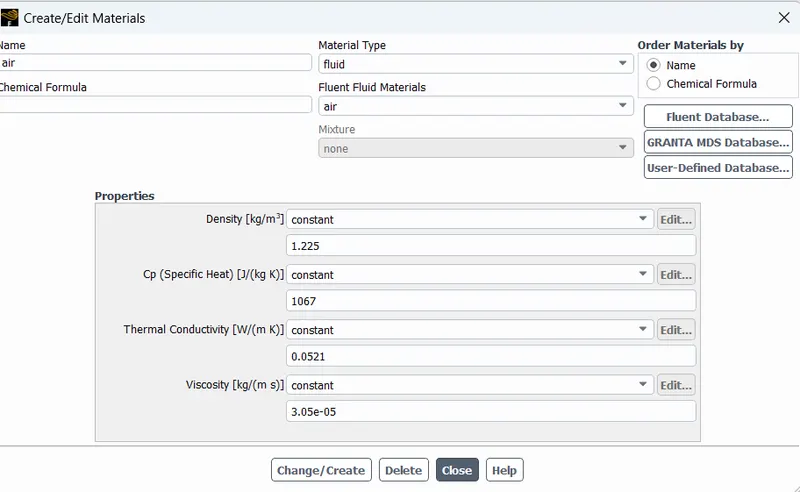
>Enable the energy equation

>choose model k-omega sst model

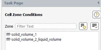
>go to cell zone condition.

>change solid volume to solid and material as alluminium

>change fluid volume to fluid and material as air

>go to boundary condition

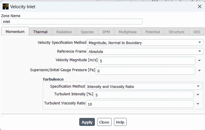
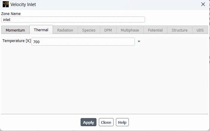
>select inlet provide velocity as 5m/s and temprature as 700k

>select outlet and check wheather the pressure is a guage 0 and temprature to 300k

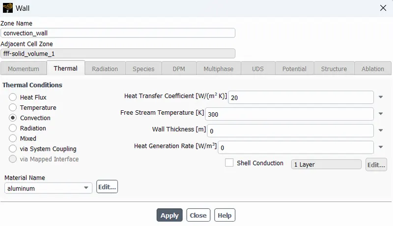
>go to convectional wall>thermal choose convection and give value of convective heat coefficient as 20 Watt/m^2k

now we create the definations

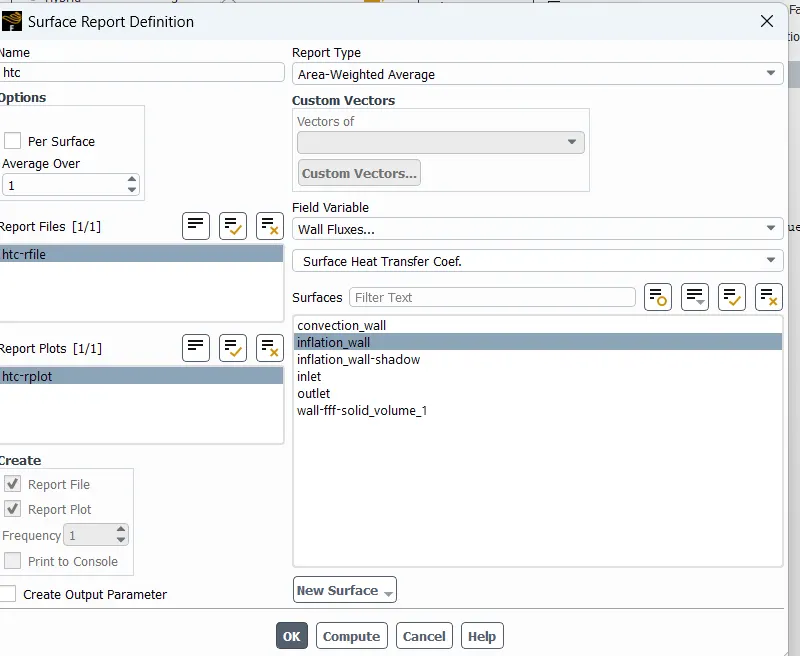
for 150mm mesh length

for 100mm mesh length

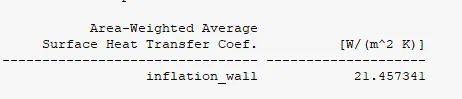
for 50mm mesh length

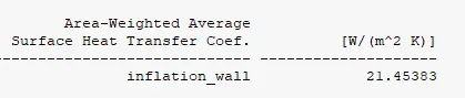
Results

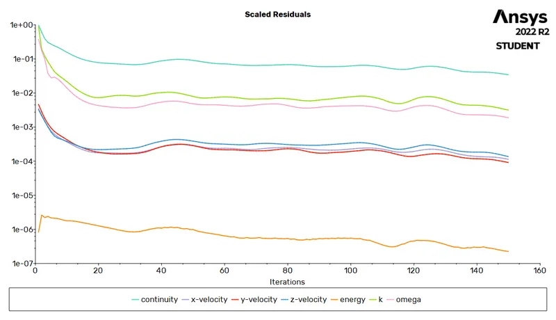
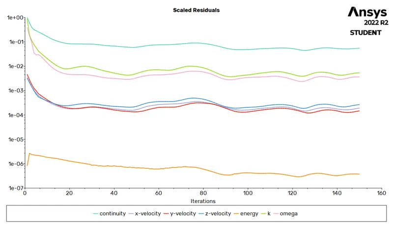
1. Residuals

Mesh Length 150	Mesh length 100	Mesh Length 50

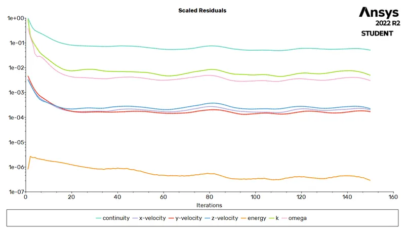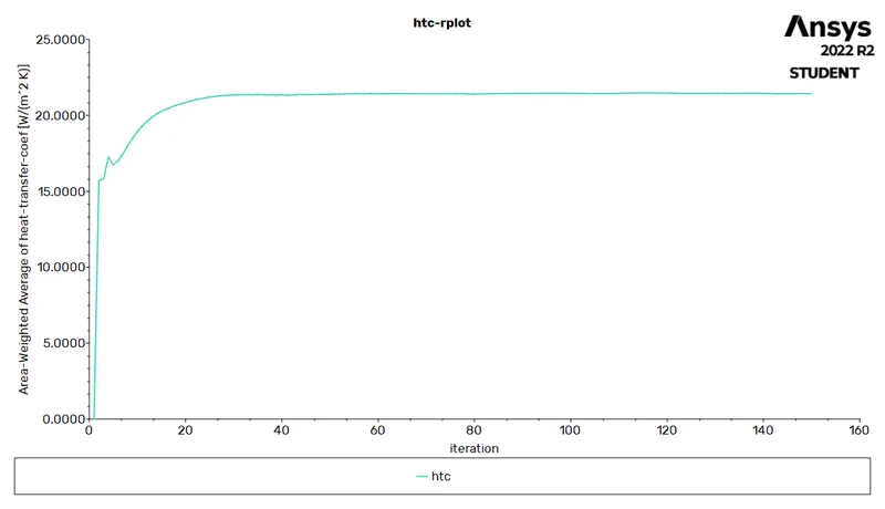
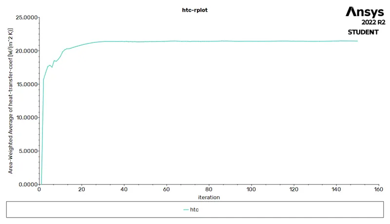
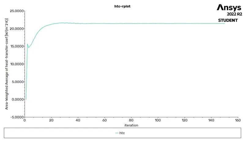
2. Convective Heat Transfer Coefficient

Mesh Length 150	Mesh length 100	Mesh Length 50

3. Y+

Mesh Length 150	Mesh length 100	Mesh Length 50

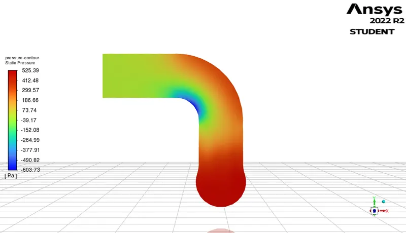
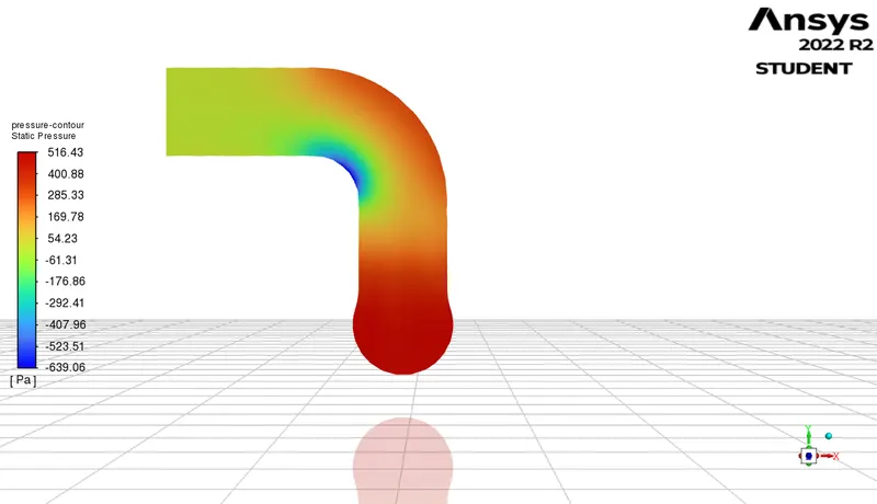
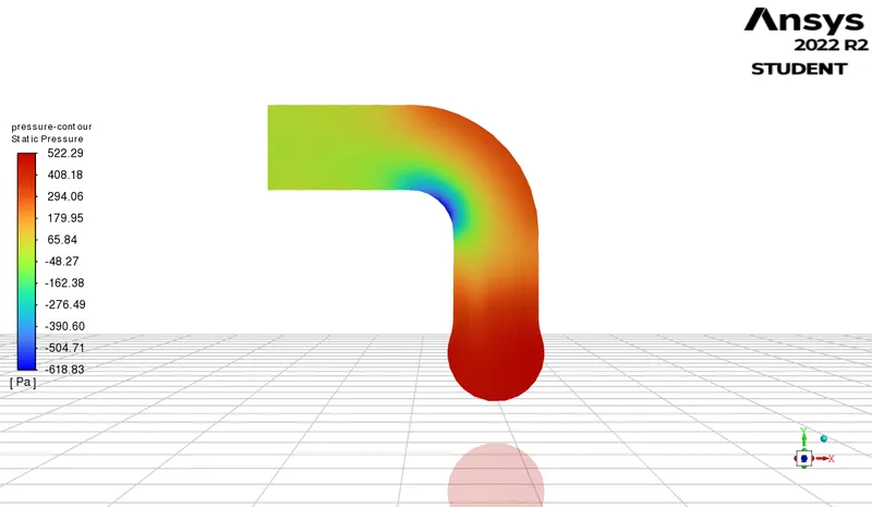
4. Pressure Contour

Mesh Length 150	Mesh length 100	Mesh Length 50

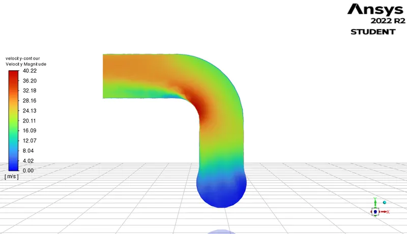
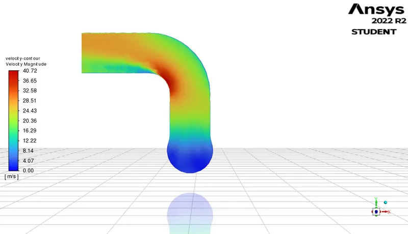
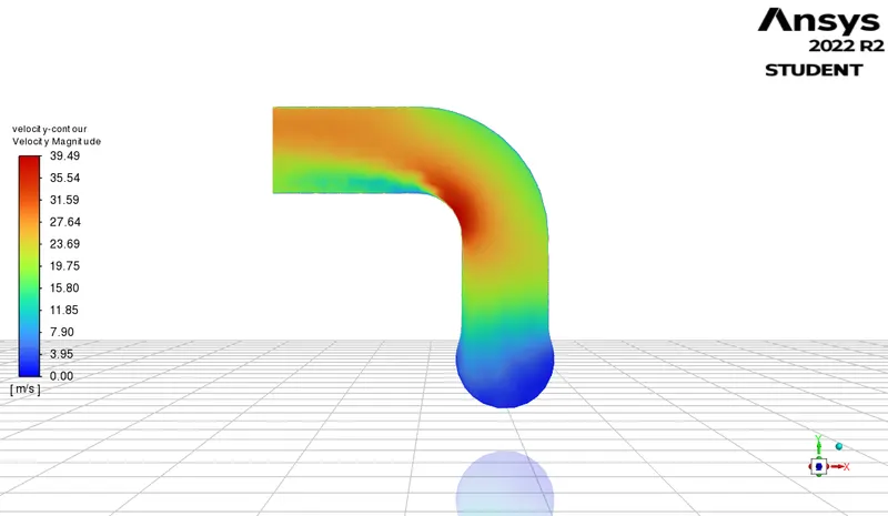
5. Veloity Contour

Mesh Length 150	Mesh length 100	Mesh Length 50

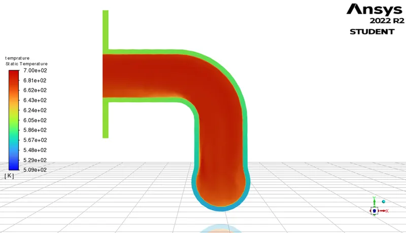
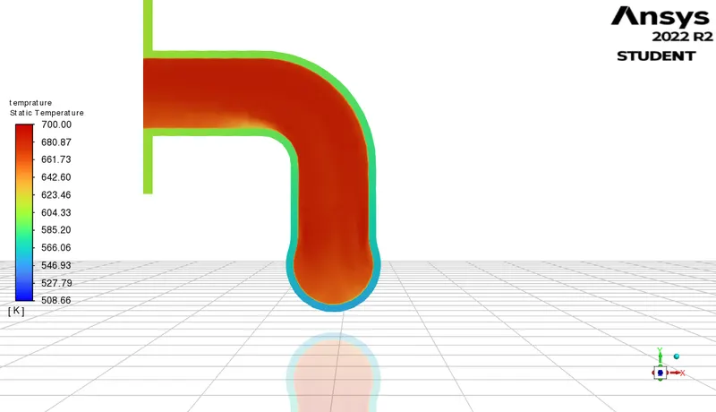
6. Temprature Contour

Mesh Length 150	Mesh length 100	Mesh Length 50

7. HTC Contour

Mesh Length 150	Mesh length 100	Mesh Length 50

8. Streamlines

Mesh Length 150	Mesh length 100	Mesh Length 50

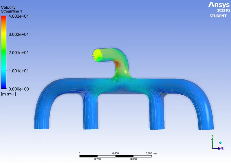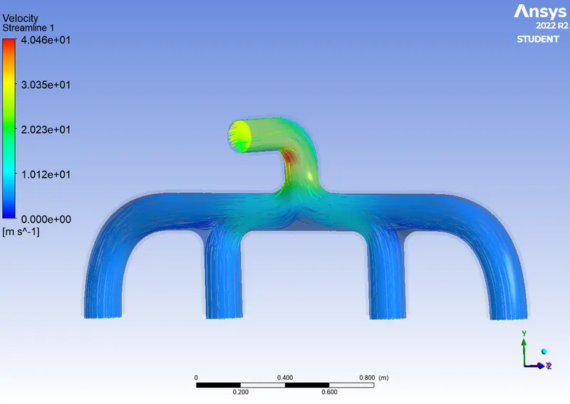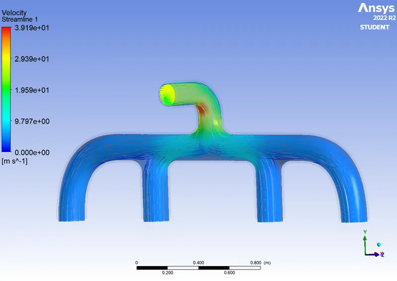Full coutour

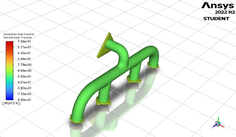
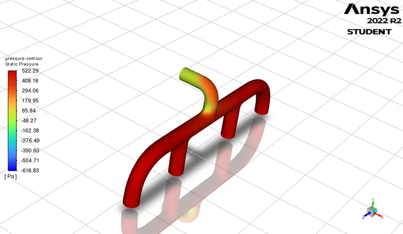
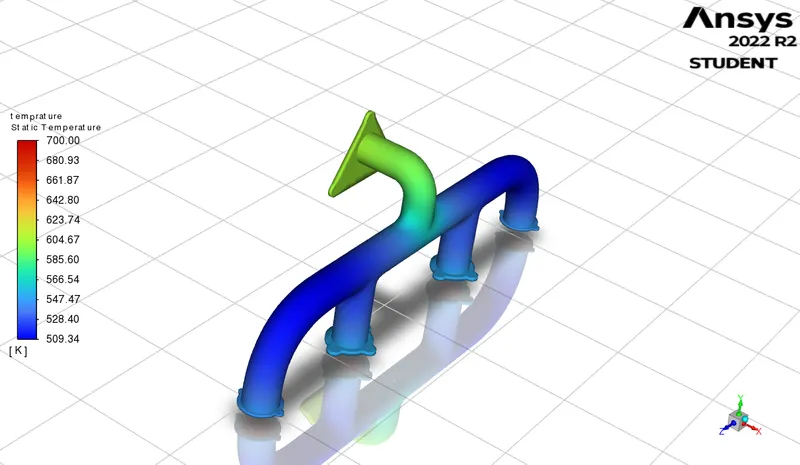
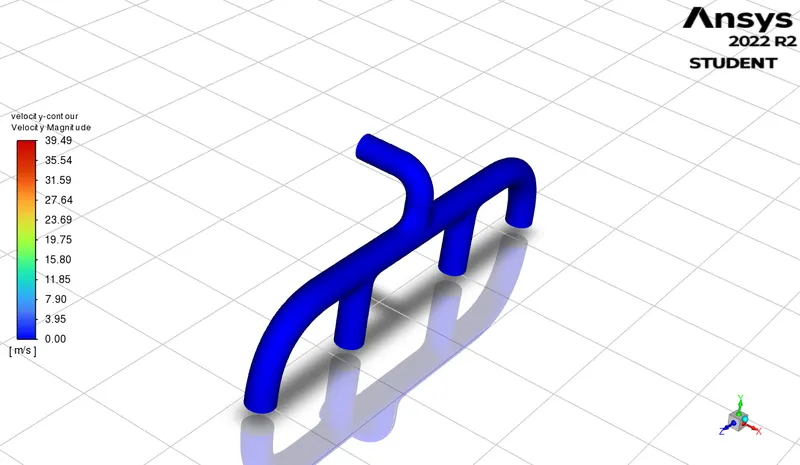
Volume rendering

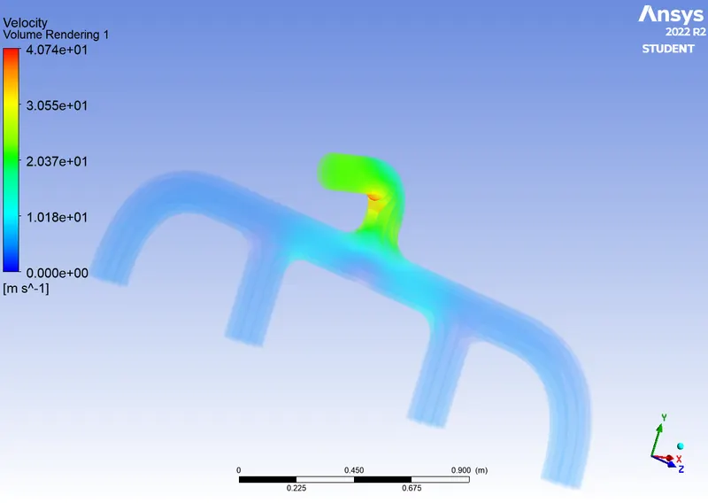
Final Results

comparsion of heat conductive coefficient

Cases	Analytical	Simulation
Mesh length 150	20.03	21.441697
Mesh length 100	20.03	21.457341
Mesh length 50	20.03	21.453830

Inference

1. Pressure is high where are the four stream meet and gradually decreases towards outlet

2. Velocity is maximun at the outlet as it having a opening to atmosphere

3. temp is maximun at outlet because all the streams meeting and result in increase the overall temprature as it obey the mass conservation

4. convective heat transfer coefficient is hight at outlet becuase from there it is exchanging more amount of heat