Week 4 - CHT Analysis on Exhaust port

AIM: -

A. To Perform a CHT Analysis on the given Exhaust Port with proper y+ values and explain the proper theory.

B. To Calculate the Heat Transfer Coefficient on the internal Surface and to verify its accuracy.

Given: -

A. The Given CAD Model of The Exhaust Port: -

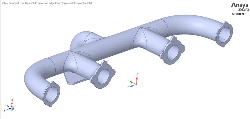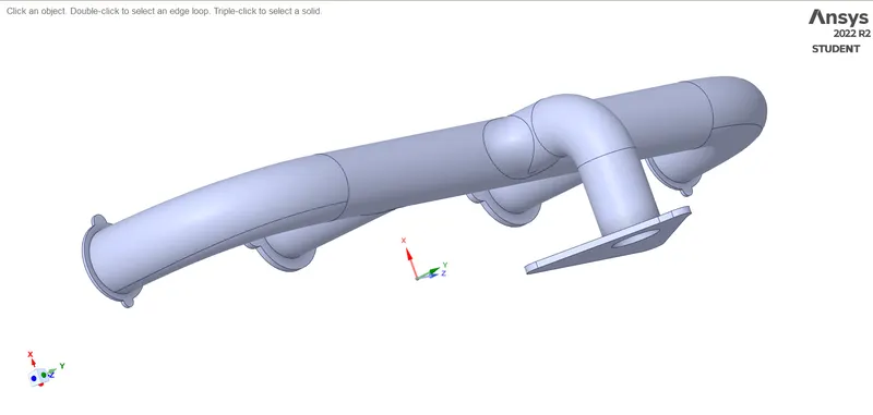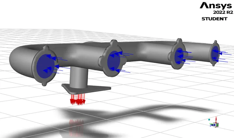
B. Conditions at Inlet, Exhaust Port Walls, and Outlets

i. At Inlet: -

a. Velocity of Fluid at Inlet `->` 5 m/sec

b. Temperature of Fluid at Inlet `->` 700 K

b. Material of Fluid `->` Air

ii. At Exhaust Port Walls: -

a. Convective Heat Transfer Coefficient of Outer Wall `-> 20 W/(m^2K)`

b. Temperature of Fluid moving around Outer Wall `->` 300 K

c. Material of the Exhaust Port `->` Aluminum

iii. At Outlet: -

a. Pressure at Outlet `->` 101.135 KPa or 1 atm

Theories: -

A. Conjugate Heat Transfer: -

A Conjugate Heat Transfer is a system where there is Heat Transfer between Solid and Fluid in the form of Convection(in the Fluid) and Conduction(in the Solid) Heat transfer.

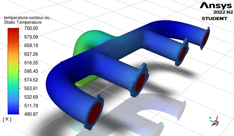
In our Current System, the Fluid is entering from 4 inlets with a Velocity of 5 m/sec and a Temperature of 700 K. The Convectivective Heat Transfer coefficient of Free stream Air is `20 W/(m^2K)` and the Material of the Exhaust Port is Aluminum. Our Study here is Focused on Analyse of the Heat Transfer Rate between Fluid and Solid and deriving the Average Heat Transfer Coefficient for the Fluid flowing within the Exhaust Port.

B. Y+ Boundary Layer: -

In a Turbulent Flow Condition, the domain of the fluid layer affected by the Viscous effect is small but very significant and these Viscous effects are very dominant in a very small region of flow from the Walls. To capture these Viscous Effects with high accuracy the Y+ Boundary layer is used.

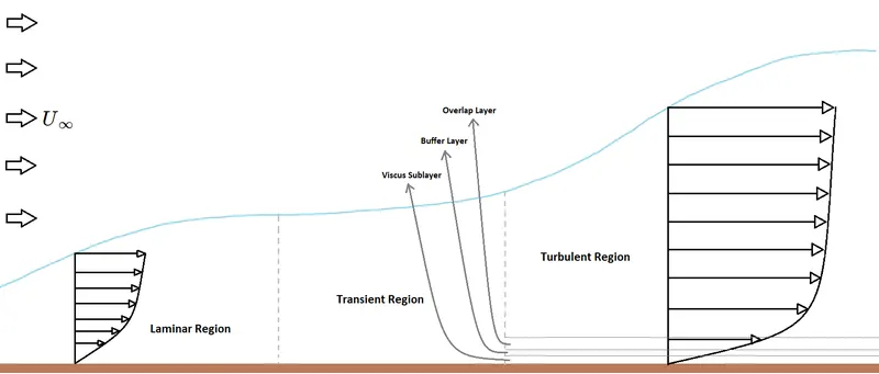
Fig.1 Diagram Represents Flow over A flat Plate(This image is inspired/Re-created from Fluid Mechanics: Fundamentals and Application, author Y. Cengel for study purposes only and with no intention to infringe the Copyright of the original Author and/or the Publication)

Y+ is a Dimension-less Number that is used to determine the thickness of the mesh layer just over the Solid Body so that the flow parameters are calculated with high accuracy.

`y+ = (rhou_(tau)triangley)/mu`

Now,

As `v = mu/rho`

`=> y+ = (u_(tau)triangley)/v`

`y+ = (rhou_(tau)triangley)/mu or (u_(tau)triangley)/v`

where, `rho ->` Density of Fluid

`u_(tau) ->` Shear Velocity

`triangley ->` Boundary Layer Thickness at that Location

`mu ->` Dynamic Viscosity

`v ->` Kinematic Viscosity

B. K-Omega SST Turbulence Model: -

This is a hybrid Model which has the features of the K-Omega and K-Epsilon Turbulence Modeling that uses the K-Omega Model closer to the wall and by switching uses the K-Epsilon Model near the free stream.

As in the current system the fluid is Moving with about 5000 Reynolds Numbers inside the Exhaust Port which is a turbulent flow condition and there is the presence of Convective heat transfer between the Fluid to the Solid. So the K-Omega SST Model is used as the Turbulence effect can be well calculated using the K-Epsilon Model and the K-Omega will be used to calculate the Convective Heat Transfer between the Fluid and Solid Interface.

Steps to Setup the Conjugate Heat Transfer Analysis of Exhaust Port: -

A. Setting up the Ansys Workbench: -

Ansys Workbench `->` ToolBox `->` Analysis System `->` `ubrace("Fluid Flow(Fluent)")_("Selecting" -> "Holding" -> "Dragging and Drooping to Project Schematic")`

B. Opening SpaceClaim Geometry and Extracting Volume: -

i. Steps to Open SpaceClaim: -

Ansys Workbench `->` Project Schematic `->` Project `->` Geometry `->` Right-Click `->` Select SpaceClaim Geometry

ii. Steps to Load the Exhaust Port Geometry: -

SpaceClaim `->` File `->` Open

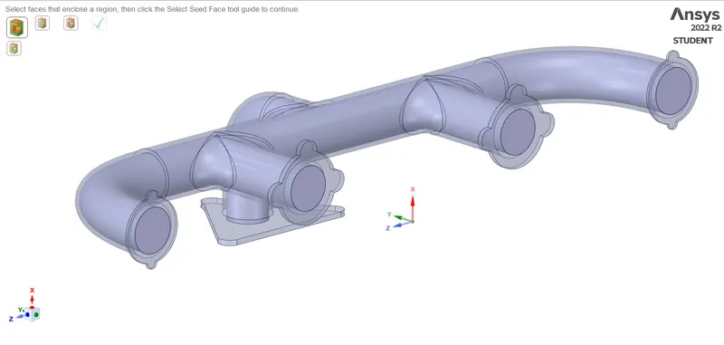
iii. Steps to Extract Volume: -

SpaceClaim `->` Prepare `->` Volume Extract `->` Select Edges `->` Enter

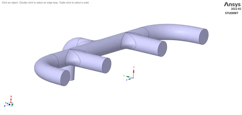Fluid Volume	Solid and Fluid Volume

Fig.2 Fluid Volume Extraction in Ansys

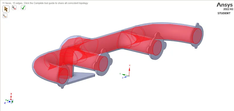
iv. Steps to Share Topology between the Solid and Fluid: -

SpaceClaim `->` Workbench `->` `ubrace("Share")_("It will auto-detect the Common Boundaries")` `->` Enter

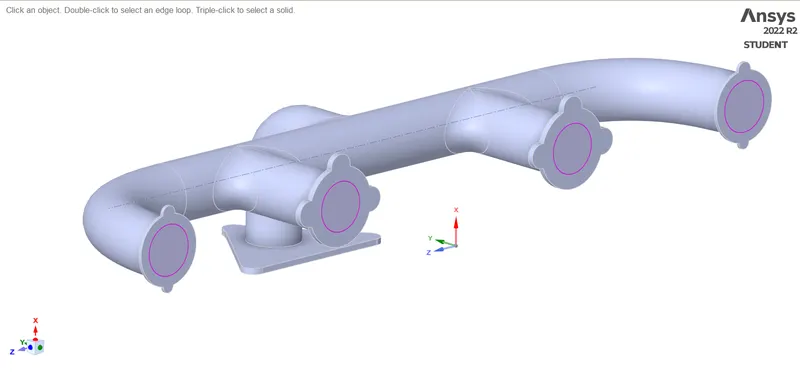Contact Areas between Solid and Fluid	Generated Share Topology

Fig.3 Sharing Common Areas of Solid and Fluid

C. Opening Mechanical(Meshing) and Meshing the Geometry: -

i. Steps to Open Meshing: -

Ansys Workbench `->` Project Schematic `->` Project `->` Mesh `->` Right-Click `->` Edit

ii. Steps to Name the Boundary: -

Mechanical(Meshing) `->` Model Working Window `->` Select the Boundary `->` Click N `->` Give the desired Name `->` Enter

a. Fluid Domain Namings: -

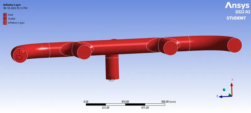
Fig.4 Fluid Domain Namings

b. Solid Domain Namings: -

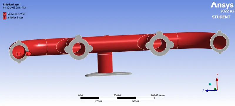
Fig.5 Solid Domain Namings

ii. Steps to Create the Mesh: -

a. Setting Base Mesh Size: Outline Window `->` Select Mesh `->` Details of Mesh Window `->` Defaults `->` Element Size is set to the desired Value

b. Meshing the Fluid: `ubrace("Select the Desired Geometry")_("Selecting the Fluid Volume")` `->` Mesh `->` Right-Click `->` Select "Sizing" from Insert `->` `ubrace("Select the desired Mesh Parameters")_("In our Case for the Selected Geometry Define mesh Size")`

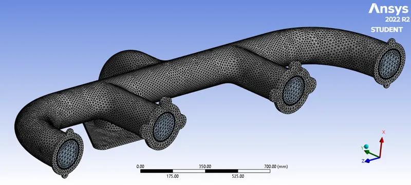
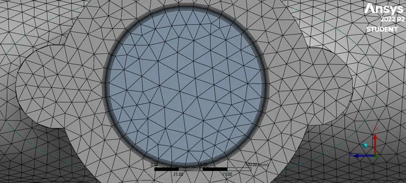
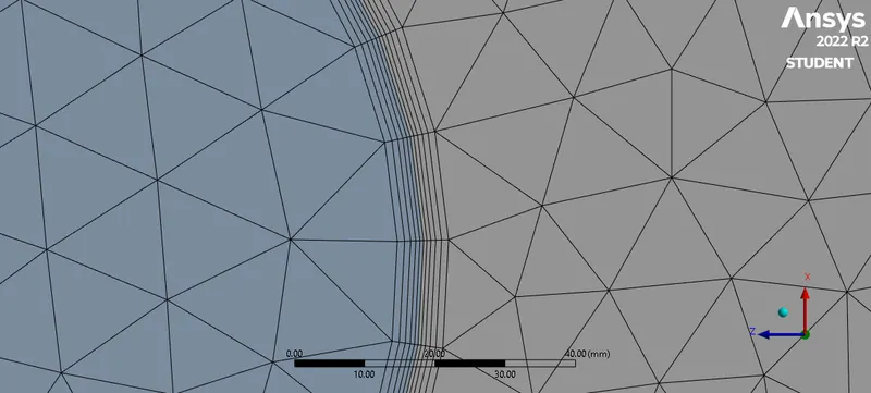
c. Creating Inflation Layer: Outline Window `->` Select Mesh `->` Details of Mesh Window `->` Inflation `->`Select "All Faces in Chosen Named Selection" from Use Automatic Inflation `->` Selected "Inflation Layer" from Named Selection `->` Select "First Layer Inflation" from Inflation Option `->` Define First Layer Thickness to 0.5mm `->` Define Maximum Layers to the desired number of layers

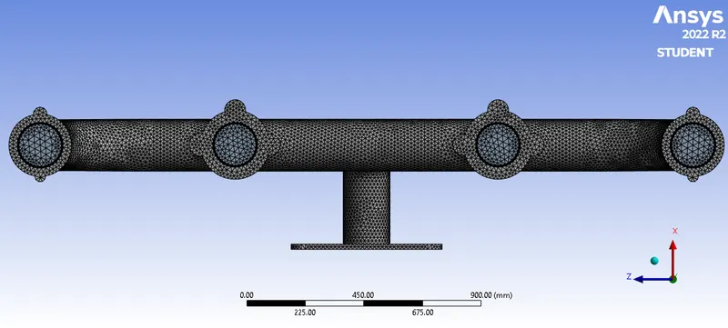Solid and Fluid Volume Meshed	Solid and Fluid Volumes Meshed - Front View
Inflation Layers	Inflation Layer - Close View

D. Setuping the Physics and Boundary Conditions: -

i. Steps to Open Ansys Fluent: -

Ansys Workbench `->` Project Schematic `->` Project `->` Setup `->` Right-Click `->` Edit

ii. Steps to Check Mesh: -

Fluent `->` Outline View Window `->` Setup `->` General `->` Mesh `->` Check

iii. Steps to Set up the Physics: -

a. Setting Viscous Solver: Fluent `->` Physics `->` Models `->` Viscous `->` `ubrace("Select Desired Viscous Model")_("In our case Select K-Omega and SST")`

b. Setting Energy Equation: Fluent `->` Physics `->` Models `->` Select "Energy"

iv. Steps to Set up Boundary Condition: -

Fluent `->` Physics `->` Zone `->` Boundaries `->` Select the desired Component `->` Select the Desired Type for that Component `->` Edit `->` Add the Values for the Component `->` Apply & Close

v. Steps to Set up Reports: -

Fluent `->` Solution `->` Reports `->` Definition `->` New `->` Select the Desired Report `->` Rename the Report `->` Change the Field Variable to Desired Variable `->` Select the desired Surface `->` Ok

vi. Steps to Initialize and Set Desired Graphical Views: -

a. Initializing: Fluent `->` Solution `->` Initialization `->` Initialize

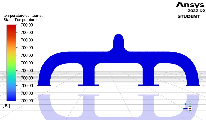
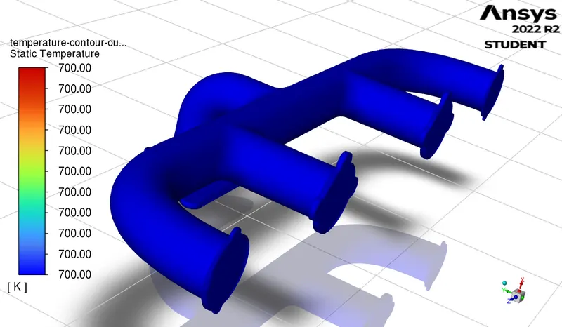
b. Setting the desired Contour: Fluent `->` Results `->` Graphics `->` Contours `->` New `->` Rename `->` Select Variable for Contour of `->` Select Surface `->` Save/Display

c. Setting the desired Vectors: Fluent `->` Results `->` Graphics `->` Vectors `->` New `->` Rename `->` Select Variable for Vectors of `->` Select Surface `->` Save/Display

d. Setting the desired Pathlines: Fluent `->` Results `->` Graphics `->` Pathlines `->` New `->` Rename `->` Select Style and give its parameters `->` Select Color of `->` Select Surface `->` Save/Display

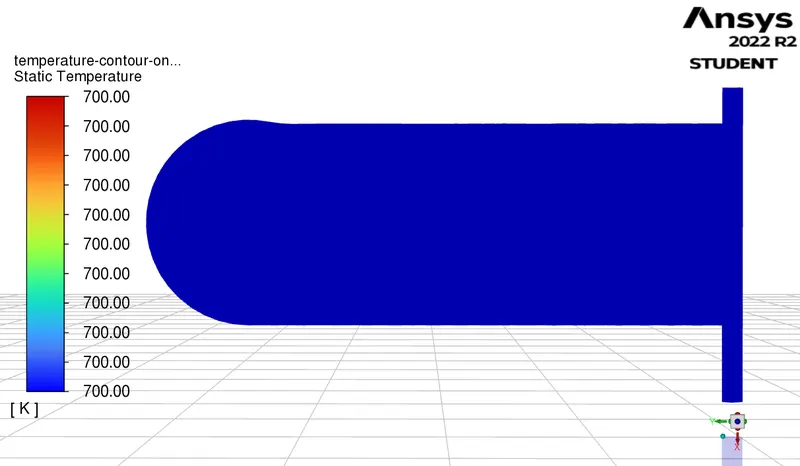
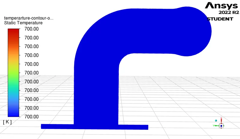
Temperature Contour of All Inlets	Temperature Contour of Outer Body
Temperature Contour of One Inlet	Temperature Contour of Outlet

Steps to Analyse the Conjugate Heat Transfer Analysis of Exhaust Port: -

A. Performing Calculations and Developing Results: -

i. Steps to Open Fluent: -

Ansys Workbench `->` Project Schematic `->` Project `->` Setup `->` Right-Click `->` Edit

ii. Steps to Run Calculations: -

a. Setting up no. of Iterations: Fluent `->` Solution `->` Run Calculations `->` Setting Desired Iterations in "No. of Iterations"

b. Running Calculations: Fluent `->` Solution `->` Run Calculations `->` Calculate

Results and Plots Generated: -

A. For Fine Mesh with Inflation Layer: -

i. Plots Developed While Calculations: -

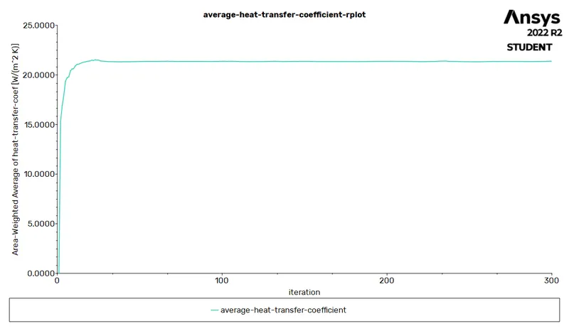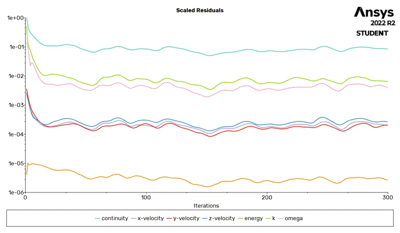
Residuals Plot	Average Heat Transfer Coefficient
Average Outlet Temperature	Outlet Temperature Standard Deviation

ii. Results Developed after Calculations: -

a. Temperature Results: -

Temperature Contour for All Inlets	Temperature Contour for One Inlet
Temperature Contour for Outer Body	Temperature Contour for Outlet

b. Pressure Results: -

Pressure Contour for All Inlets	Pressure Contour for Outlet

c. Velocity Results: -

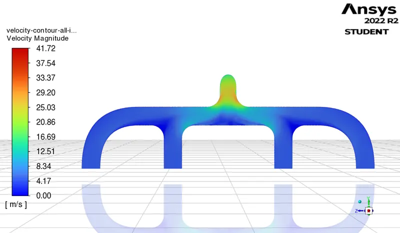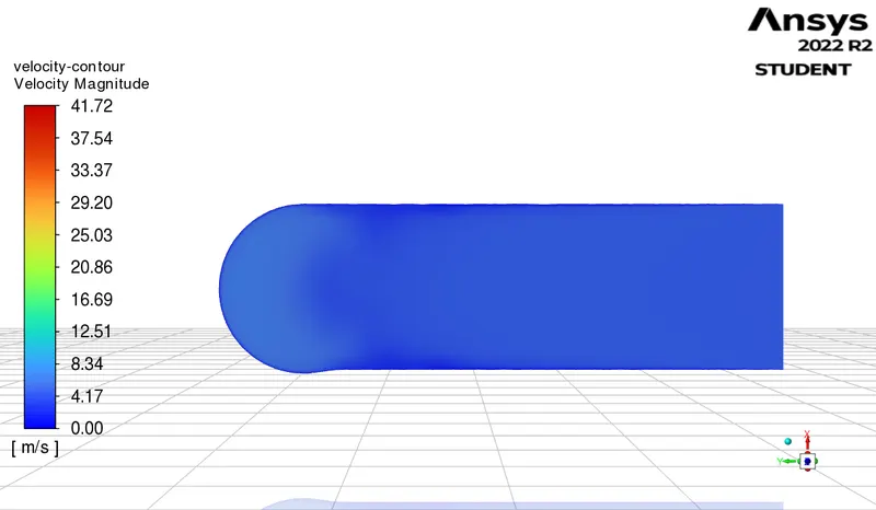Velocity Contour for All Inlets	Velocity Contour for One Inlet
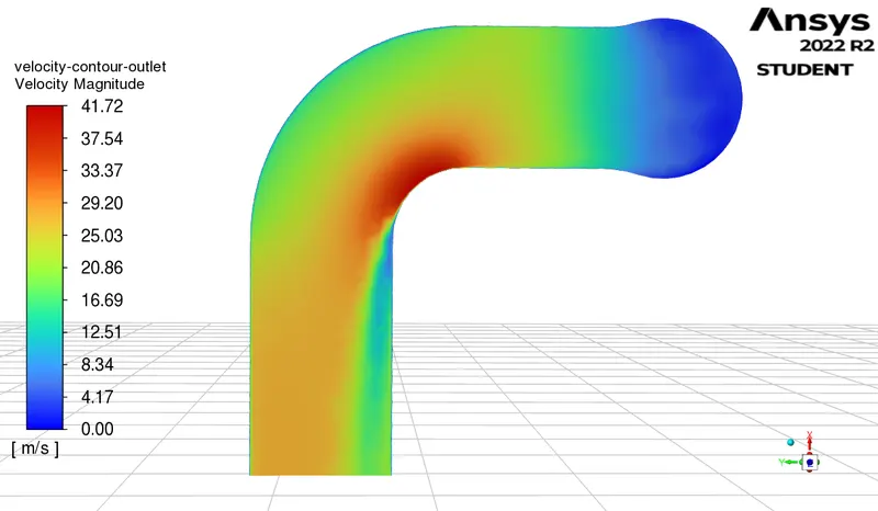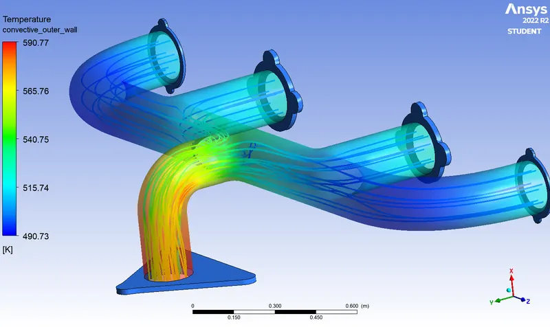Velocity Contour for Outlet	Velocity Pathlines with Temp. Contour for System

B. For Course Mesh with Inflation Layer: -

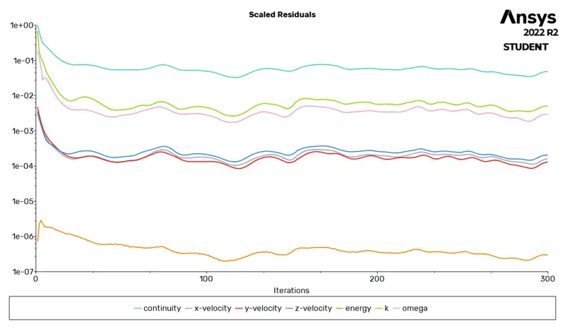
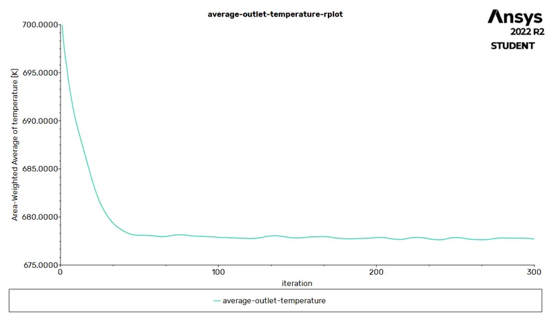
i. Plots Developed While Calculations: -

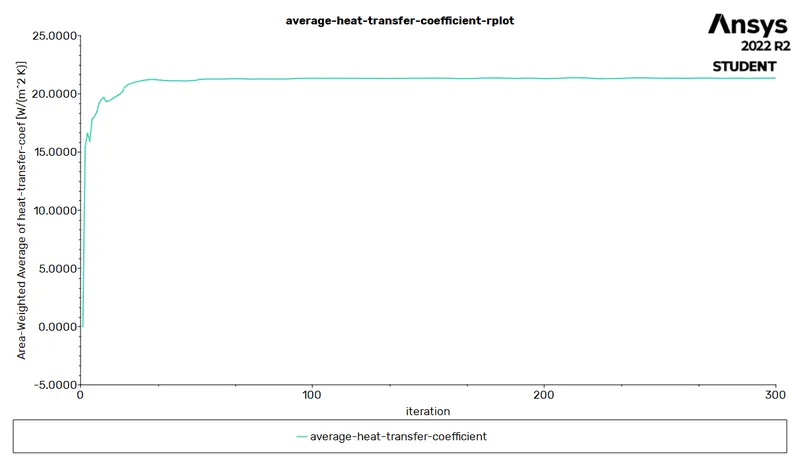Residuals Plot	Average Heat Transfer Coefficient
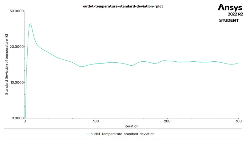Average Outlet Temperature	Outlet Temperature Standard Deviation

ii. Results Developed after Calculations: -

a. Temperature Results: -

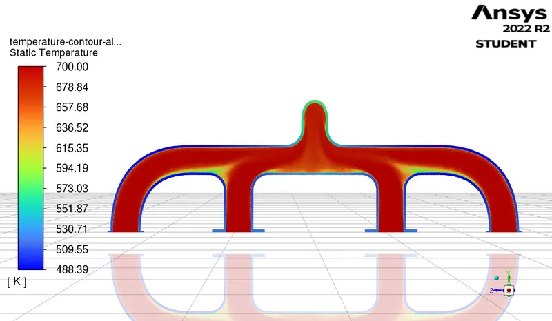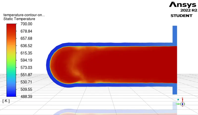Temperature Contour for All Inlets	Temperature Contour for One Inlet
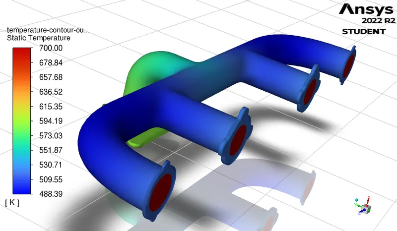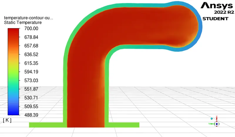Temperature Contour for Outer Body	Temperature Contour for Outlet

b. Pressure Results: -

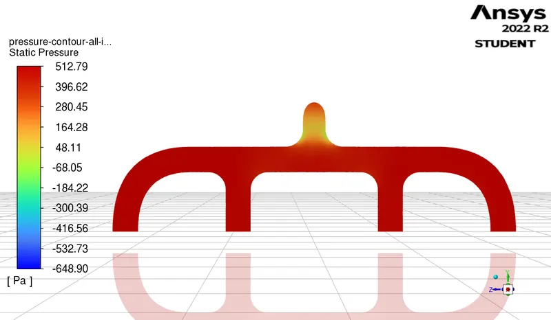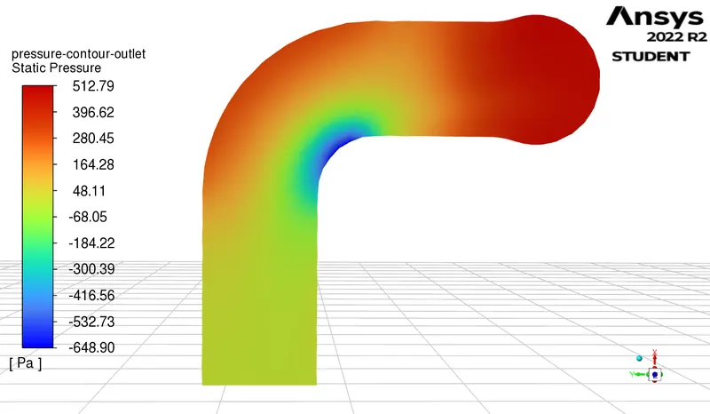Pressure Contour for All Inlets	Pressure Contour for Outlet

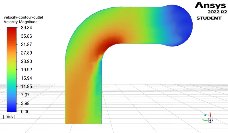
c. Velocity Results: -

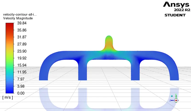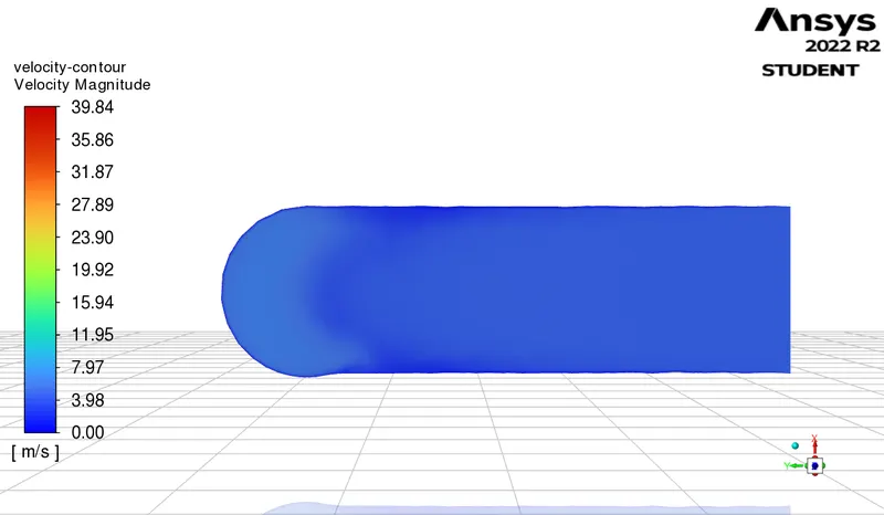Velocity Contour for All Inlets	Velocity Contour for One Inlet
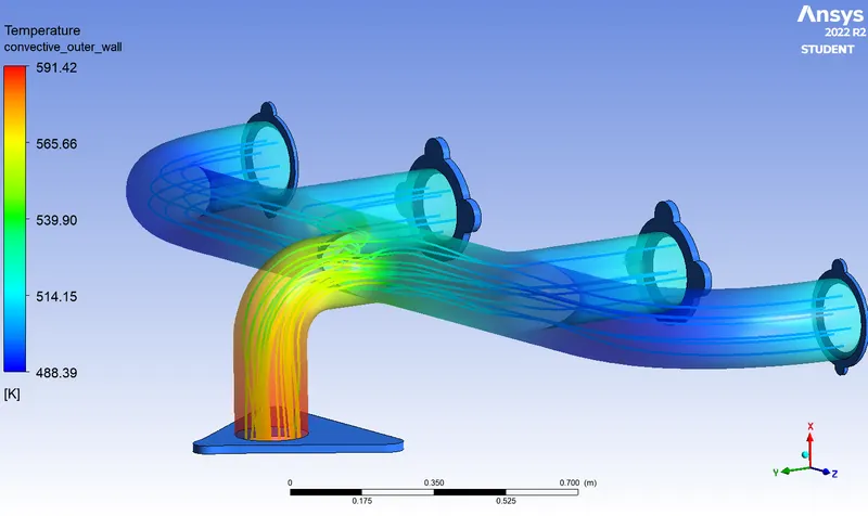Velocity Contour for Outlet	Velocity Pathlines with Temp. Contour for System

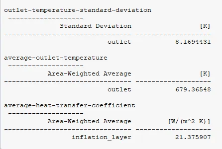
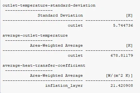
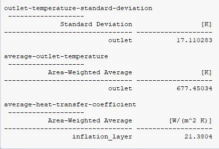
C. Results Generated by different Mesh sizes: -

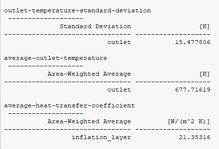Course Mesh Without Inflation	Course Mesh With Inflation
Fine Mesh Without Inflation	Fine Mesh With Inflation

Average Heat Transfer Coefficient of the inlet Fluid `= 21.38 W/(m^2K)`

Observations and Reasons: -

A. Mixing Efficiencies of the Fluid and its effect on heat transfer: -

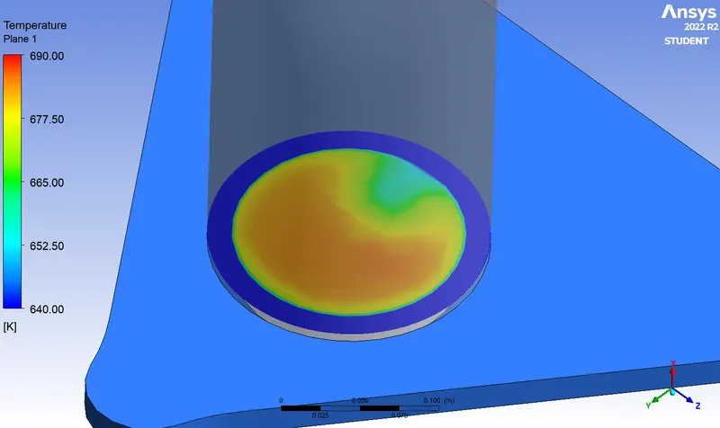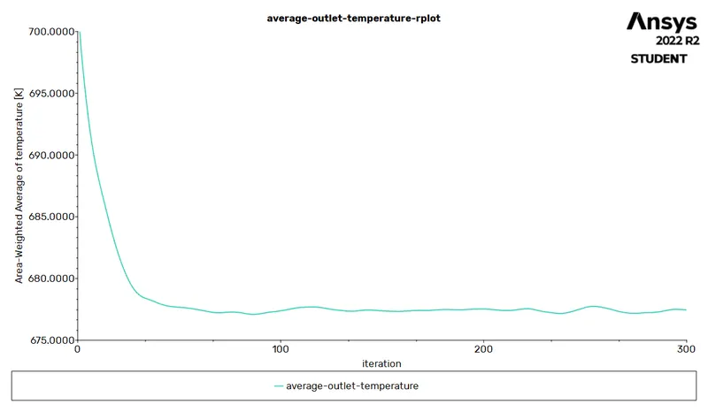
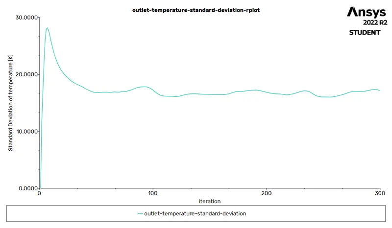
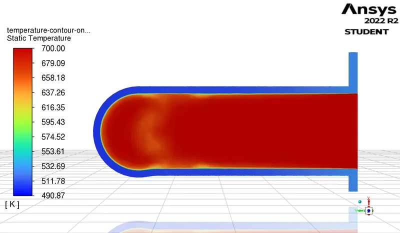
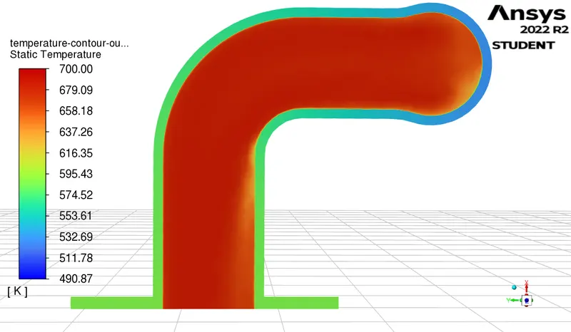
In the First Observation, it can be seen that the Standard Deviation of Temperature at the Outlet for Inflation Layered Mesh is 17 which implies that the uniformity of temperature at the outlet is not there and indicates that there is a gradient of Temperature from the mid of the Fluid Volume to the Periphery of the fluid Volume, Which is responsible for the High Rate of Heat Transfer between the Fluid to the Solid	In the Second Observation, it can be seen that the Temperature Profile has a distribution of Hot Fluid at the center to relatively cold fluid at the periphery of the Fluid but with a slight deviation of the Temperature at one side which is because the bend in the pipe which causes a Slow moving Fluid region with a high number of eddies formation and as the other region near it is turbulent this is leading to a Very High heat transfer coefficient at that region
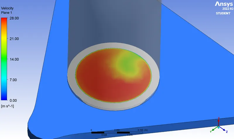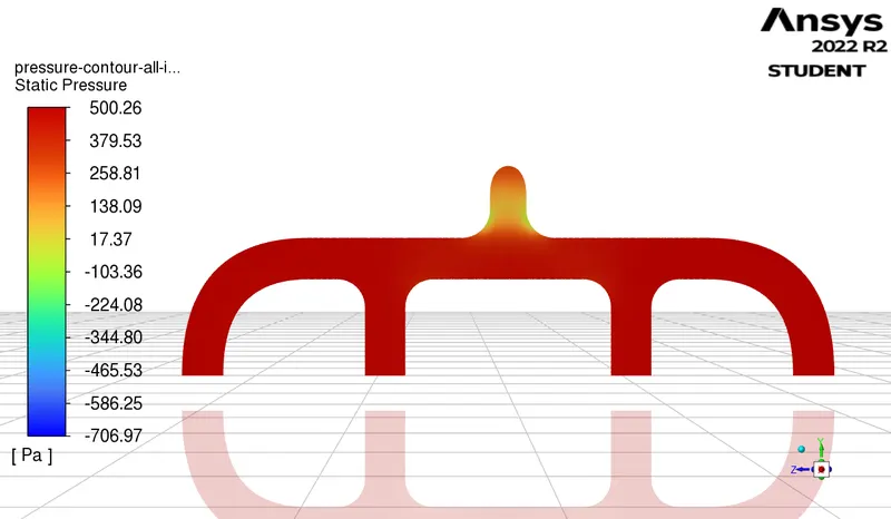
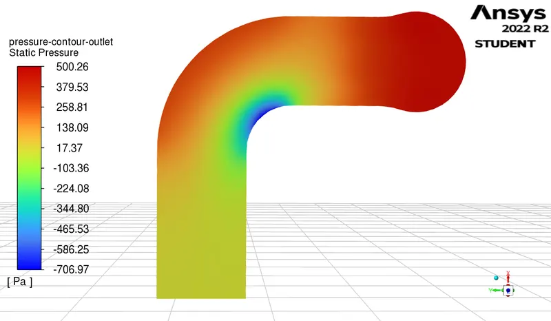
It can be observed that there is a high velocity at the Outlet which is causing high turbulence at the Outlet which is the reason for the high heat transfer coefficient at the Outlet	It can be observed that there is a slow-moving region of fluid at a region at the Outlet which is due to the bend in the flow field this region is slow-moving and has eddies formed in the region which is causing a high value of heat transfer coefficient.

B. Reasons to Accept the Simulation Results: -

The following are a few reasons that indicate the accuracy of the Results: -

i. As the Heat Transfer is Observably very high at the Outlet. The Velocity at the Outlet is high and as the Fluid, until the Outlet has already suffered a lot of bends which is responsible for the formation of Eddies that move along the Fluid, and the Heat Transfer Increases as these eddies also move along high-Velocity Fluid.

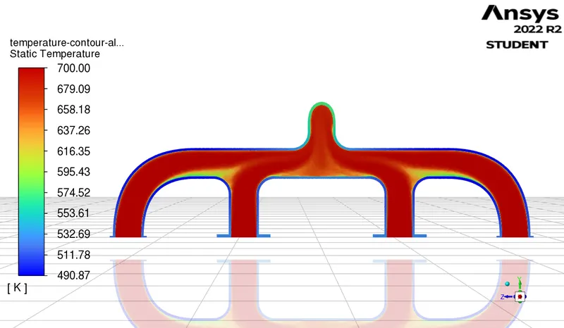
ii. The Temperature and Velocity Profiles that are formed at each point in the System. It can be observed that the region where the fluid is experiencing a backflow or vortex those regions experiences a high Heat transfer Coefficient.

iii. As the Fluid is moving with a substantial Velocity there is good mixing of fluid within the System but there is no extreme Outward Heat Flow between the Fluid and Solid because the Cross-Sections Shape of the Exhaust Port is Circular Which means there is not enough Area of Fluid in contact with The Solid to have a high amount of heat transfer. This can be seen in the inlet regions where the Walls of the Solid are not rising in temperature to any significant amount.

Click Here to Download the Ansys Files for this Challenge