Week 4 - CHT Analysis on Exhaust port

Notice: - After the analysis, the size of the file is more, but in the challenge submission time it is not supported because of its large so I am sharing the google drive link please download from the link.

Link:

https://drive.google.com/file/d/1YO5DFtgJOPx6wHP7Vxd-h4dSnE0uVWim/view?usp=sharing

Conjugate heat transfer

By transferring thermal energy at their interfaces, the Conjugate Heat Transfer (CHT) analysis type enables the simulation of heat transfer between solid and fluid domains. The simulation of heat exchangers, the cooling of electronic devices, and general-purpose cooling and heating systems are examples of typical uses of this analysis type. Such heat transfer devices are difficult to model and build because of coupling, which calls for a sizable number of parameters to describe both the fluid and solid domains. Decoupling the issue by modelling each domain independently, then integrating the models of the two domains using the continuity conditions at the solid/fluid interface, which are:

• Continuity of temperature field
• Continuity of heat flux

Every simulation should explain how heat fluxes and temperature variations vary throughout the domain. Comparing it to the entire description requiring the solution of the energy partial differential equation, it must be a fairly basic model (PDE). However, it must also be precise enough to account for the heat flux fields and temperature fluctuation over the solid/fluid interface.

Application of CHT

A fluid stream close to an item's surface, which is not the same temperature as the fluid bulk, causes convection, a complex phenomenon that involves the transfer of energy between an object and its surroundings. The phenomenon thus possesses both a local and a global aspect. Incoming fluid close to the object is contaminated by exchanges that have already taken place at numerous locations along the boundary, giving the exchange a global character as well as a local character depending on the local object conditions at any given point. When this convection and conduction take place at the same time in this time conjugate heat transfer takes place.

Since wall heat transfer coefficients and their local changes on surfaces are directly estimated within the model rather than relying on reduced empirical estimates, the CHT approach has an advantage over FE thermal evaluations. Therefore, the CHT technique provides advantages for applications where heat transmission is either non-uniform or challenging to estimate empirically.

Maintain y+ value

In our conjugate heat transfer model, we consider the y+ value for two conditions. Y+ value for the boundary layer we are taking two y+ values for our two cases. In the first case, the y+ value is 1 where we consider the k-omega SST model and in the second case, the y+ value will be 50 where we consider a k-epsilon standard model for analysis. This y+ value is used to define the first layer distance in the inflations layer. When in our turbulence model y+ value is less than 5 we apply the k-omega model and when the y+ value is greater than 30 we apply the k-epsilon model. In our case, we tell the y+ value as 1 in the first case and 50 in the second case.

Case-1

Velocity (v) = 5m/s

Density (ρ) = 1.225 kg/m^3

Dynamic viscosity(µ) = 1.7*10e-5 kg/ms

Diameter = 0.166m

y+ = 1

After applying all these values, we will get the first layer thickness of 0.056mm and the Reynolds number is 56820.722

Case-2

Velocity (v) = 5m/s

Density (ρ) = 1.225 kg/m^3

Dynamic viscosity(µ) = 1.7*10e-5 kg/ms

Diameter = 0.166m

y+ = 50

After applying all these values, we will get the first layer thickness of 2.8mm and the Reynolds number is 56820.722.

Modelling approach

In the modelling approach we are following these steps

• Geometry setup
• Meshing
• Problem setup
• Solving
• Post processing

Geometry setup

In the geometry setup we are import the geometry in the space claim and create the fluid volume. After the separate the volume have to on the share topology for the sharing boundary which will give a better mesh.

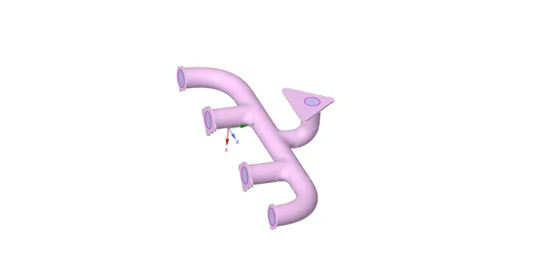
(Geometry of exhaust port)

Meshing

In the meshing tool we are using fine mesh with the element size 10mm and in two inflation layers for two conditions for two y+ value. For k-omega model we are apply y+ value as 1 and for k-epsilon model we are applying y+ value as 50. For these two y+ value we will get two first layer thickness and take 15 layers.

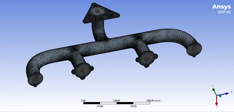
(Meshing)

In the time of sizing of mesh, we will apply the inflation layer which gives the fine boundary layer and gives the more accurate result. Before the generate mesh, we have to assign the name selection which are inlet, outlet, outer wall and the inflation layer. That inflation layer is for the convection on the outer most surface of pipe and the inflation layer ion the outer surface of the fluid volume.

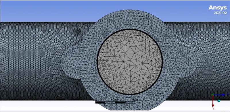
(Inflation layer)

Problem setup

In the problem setup we are applying the boundary conditions and applying the solving methods. For two cases we apply two methods k-omega method and k-epsilon method. Solving it by pressure-based solver with steady state, For solving we take 1000 iterations with hybrid initialization our boundary conditions are-

Inlet

Velocity-5m/s

Temperatre-700K

Outer wall

Convective heat transfer co efficient- 20w/m^2K

Post processing

Case-1

In the case 1 we consider the y+ value as 1 and take the k-omega SST model. The results are given in below

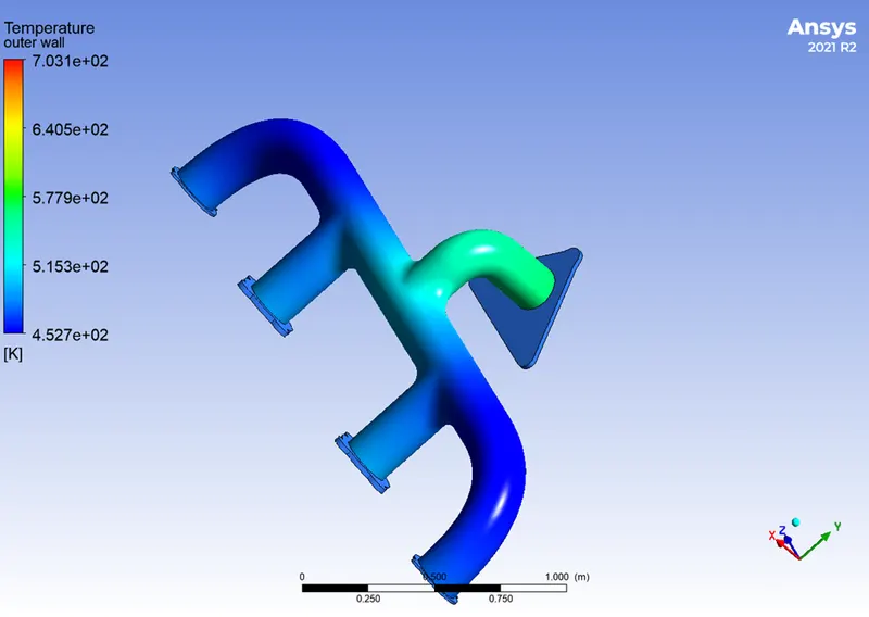
(Temperature profile from outer wall)

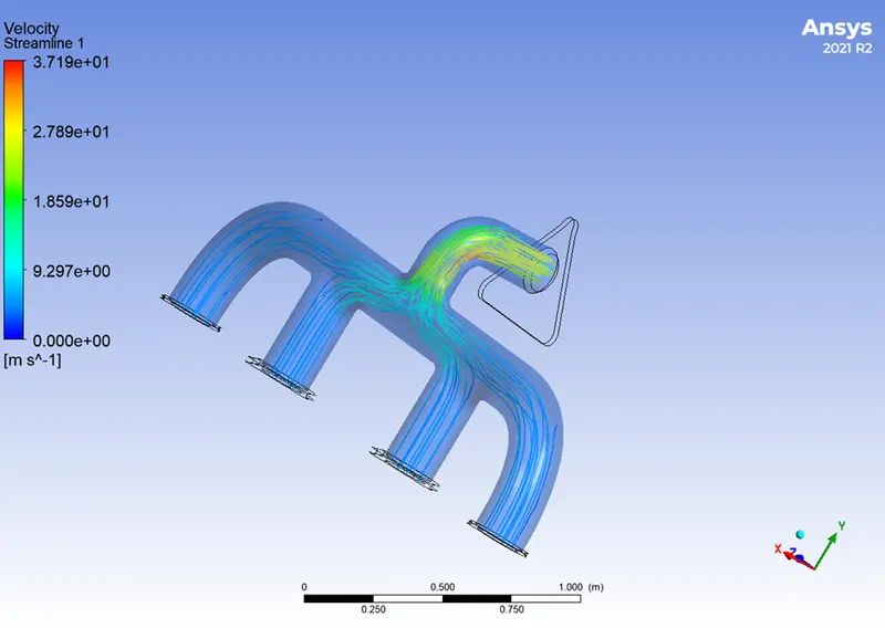
(Streamline with velocity profile)

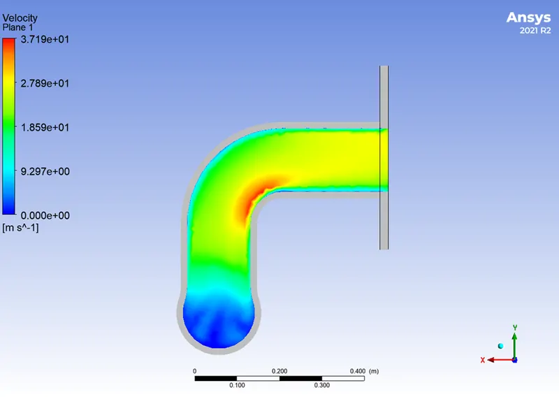
(Velocity contour plot)

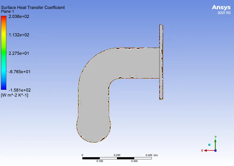
(Surface heat transfer coefficient contour plot)

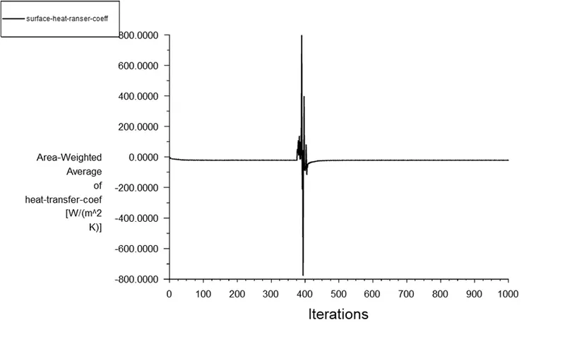
(Area weighted avg. of heat transfer coefficient)

From the above images we can see the streamline flow with velocity profile, temperature, velocity at outlet in a plane, temperature distribution in a plane and the specific heat transfer coefficient is showing. When we tale the y+ value as 1 and the first layer distance is 0.056mm and applying k-omega turbulence model. We can see the maximum heat is experienced in the outlet bend portion and velocity also more in this portion. So that the heat transfer coefficient is more is here for this more temperature is experienced. This heat is released to the room temperature so that the average specific heat transfer coefficient is in negative and value is -19.5634 W/m^2K.

Case-2

In the case 2 we take the y+ value as 50 and the solving method as k-epsilon, and analysis the results

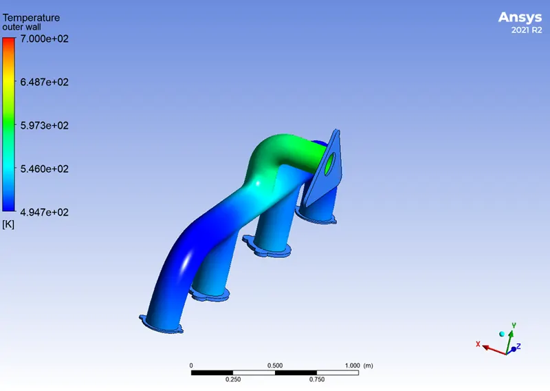
(Temperature profile from outer wall)

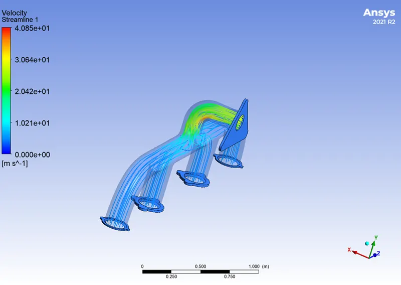
(Streamline with velocity profile)

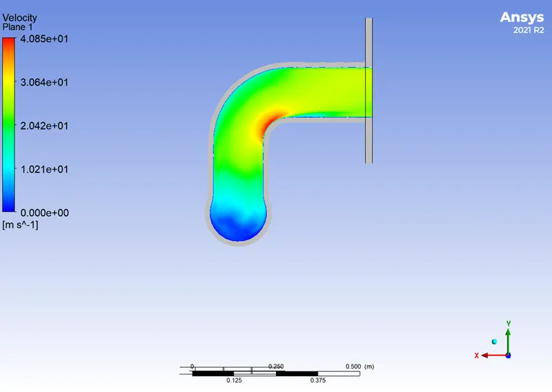
(Velocity contour plot)

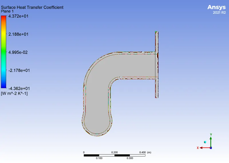
(Surface heat transfer coefficient contour plot)

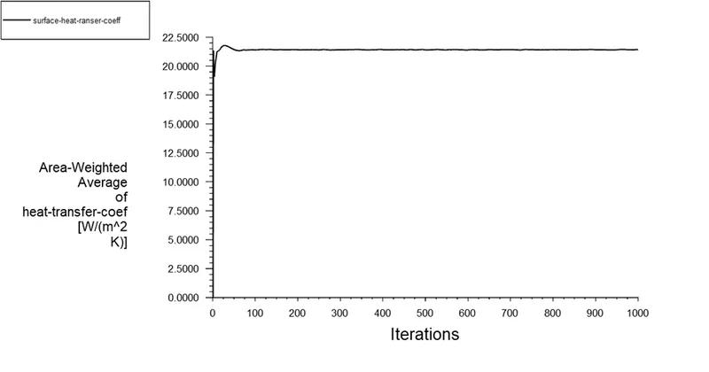
(Area weighted avg. of heat transfer coefficient)

We can see in the second case the result experienced is nearly same the velocity and temperature are increase in same place of the port. When we change the inflation layer the specific heat transfer coefficient is changed now our specific heat transfer co efficient is 21.3541W/m^2K which is positive. This is the convective heat transfer coefficient.

Prediction of HTC

We are finding two value of heat transfer coefficient now we can relate with the theoretical value of heat transfer coefficient. From the Nusselt number we can get the heat transfer coefficient

Nu=convective heat transfer/conductive heat transfer=hL/k

From this relation we can get the vale of h, for this we need Nusselt number from Reynolds number and Prandtl number relation

Nu=0.023*Re^4/5*Pr^n

Pr = Cpµ/k

K=1.4WmK

n= 0.4 for the fluid being heated and 0.3 for the fluid being cooled

from these equations we get the value of h is 19.33W/m^2K

In our two cases the heat transfer coefficient nearly equal to the theoretical heat transfer coefficient. So our prediction is correct.

Factors that accuracy of the prediction

• Target mesh length is the mot important factor of the prediction
• Y+ value for the first layer of the inflation
• The share topology for the interaction of the mesh links are most important otherwise our meshing is create some gap that reduce our heat transfer coefficient.
• Methos applying for solution is also an important factor
• Number of inflation layer gives more fine mesh
• Outer atmospheric temperature also take place when it changes heat transfer co efficient also changes.

Conclusion

In this analysis we will know about how the heat transfer coefficient changes when the factors are changes. Our simulation result is nearly equal to the theoretical result. In order to compare the numerical and CTM solutions for the same boundary conditions, a conjugate problem was addressed. On the other hand, because we do not know which or profiles are present at the interface and because there are insufficient HTC correlations for any given mix of fluid-solid domains, the HTC cannot address conjugate heat transfer problems.