Week 4 - CHT Analysis on Exhaust port

Aim: To study the CHT analysis on Exhuast port of Vehicles.

1. Give a brief description of why and where a CHT analysis is used.
2. Maintain the y+ value according to the turbulence model and justify the results.
3. Calculate the wall/surface heat transfer coefficient on the internal solid surface & show the velocity & temperature contours in appropriate areas.
4. How would you verify if the HTC predictions from the simulations are right? On what factors does the accuracy of the prediction depend on?

1. Give a brief description of why and where a CHT analysis is used.

Conjugate heat transfer is a type of heat transfer analysis between solids and fluid(s). This type of heat transfer includes both convection (between fluids) and conductive (between solids) heat transfer, as well as both forced and natural convection. Common applications and use cases of this thermal simulation type include electronics cooling, heat exchangers, industrial machinery, some AEC cases, and more. In order to demonstrate best practices for this application type, an electronics cooling application will be used as an example

Application of CHT analysis

Internal Combustion Engine:

Internal Combustion engine industry is moving toward simulating the entire system rather than independent components. The accuracy of the predicted combustion in the cylinder is dependent on the temperature boundary conditions in the cylinder. By considering heat transfer in the metal components (e.g., the cylinder head, liner, piston, etc.), the cylinder wall no longer has a user-specified temperature, but instead has temperatures predicted as part of the complete-system simulation. This makes the overall simulation results more predictive by reducing the dependence on assumed boundary conditions.

Electromobility:

Effective cooling strategies are critical for various components of emobility systems. Electric motors have high power densities and thus generate a significant amount of heat. If a motor is not properly cooled, high temperatures in the motor can cause the demagnetization of the permanent magnets and the breakdown of the winding insulation. In CONVERGE, you can analyze a range of motor cooling methods using CHT modeling, including air cooling, water jacket cooling, and oil spray cooling.

For lithium-ion battery packs, CHT simulations are necessary for conducting cooling analyses under normal operating conditions and for predicting thermal runaway. Thermal runaway occurs when a cell reaches a temperature that triggers a cascade of exothermic reactions, causing the temperature to continue to increase. CONVERGE allows you to predict if a runaway cell will cause adjacent cells to initiate thermal runaway, which can be catastrophic to a battery pack.

Aerospace:

One way to achieve higher efficiency in gas turbine engines is to increase the temperatures inside the combustor. These temperatures often exceed the melting point of the metal alloys used to construct gas turbine combustors, necessitating methods for both cooling and insulating the combustor walls. With CONVERGE, you can accurately predict the combustor wall temperatures and analyze various cooling methods, such as effusion cooling, impingement cooling, and film cooling.

Liquid rockets are another application where capturing CHT is important. As the liquid oxidizer travels from the cryogenic tanks to the combustion chamber, it simultaneously cools the device and picks up heat along the way. The properties of the oxidizer depend on the temperature, often varying from a liquid-like supercritical fluid to a gas-like supercritical fluid, which significantly affects how the oxidizer will mix upon injection into the combustion chamber. Investigating the preheating of the liquid oxidizer is essential for accurately simulating combustion down the line.

Geometry:

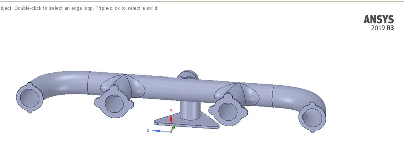
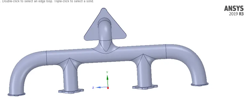
Step one import the model and perform volume extract operation on edges.

Step two share the solid and volume using shareprep option.

Geometry is same for all three cases.

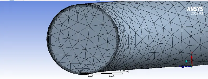
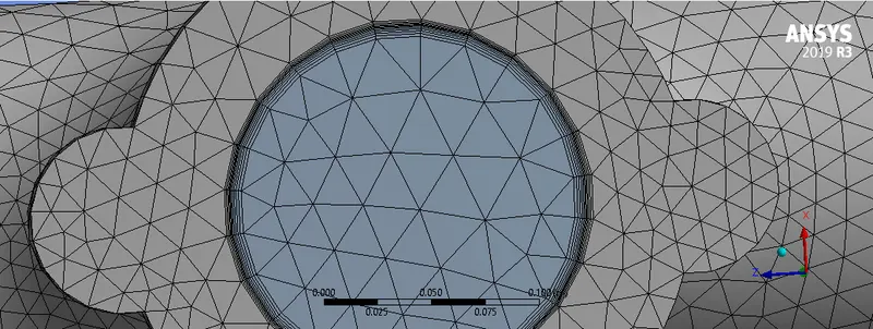
Meshing:

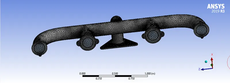
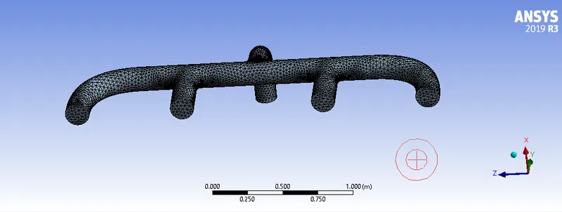
Meshing is same for all three cases.

Setup and Solution:

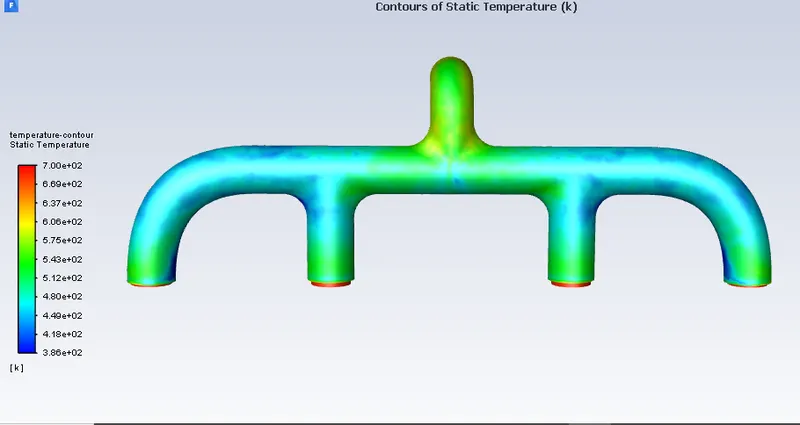
Case 1

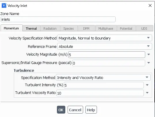
V = 5 m/s

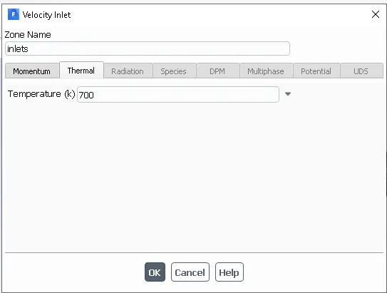
Temperature = 700 K

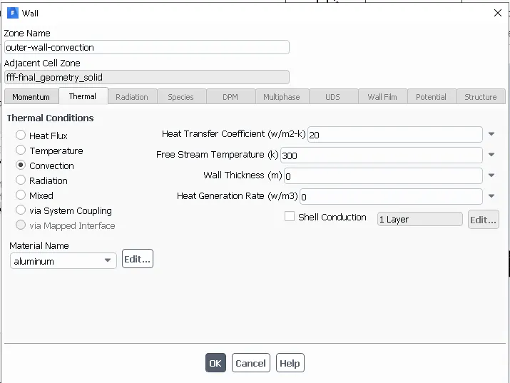
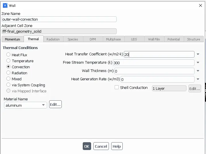
Heat transfer coefficient h = 20 W/m^2 K

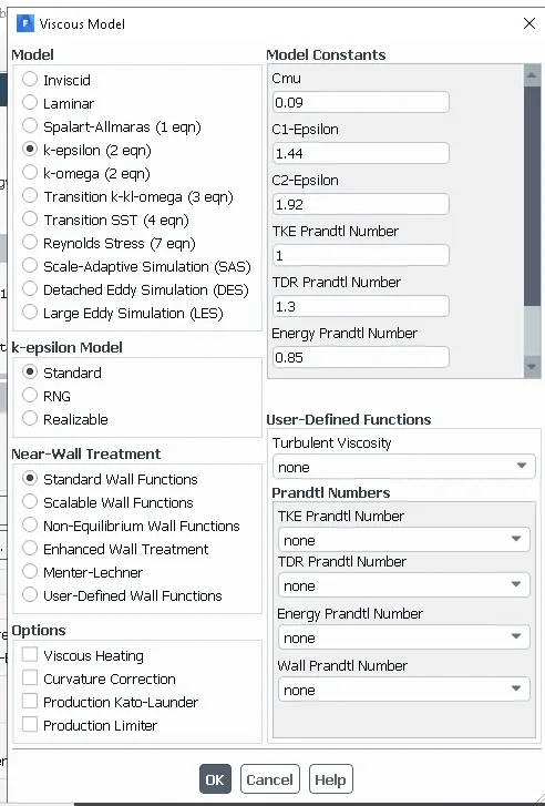
K-epsilon

Standard

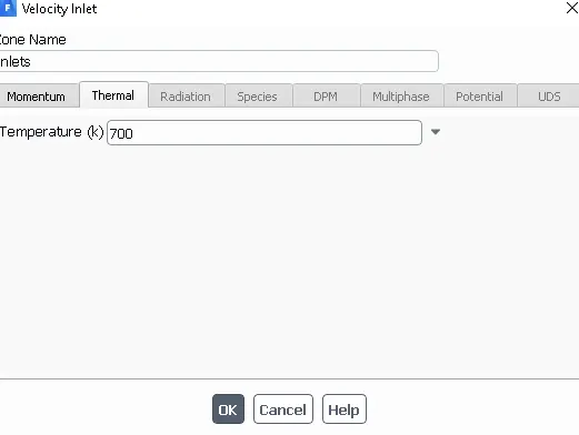
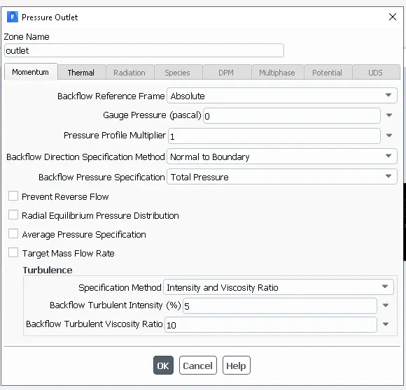
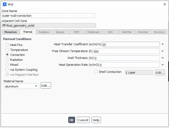
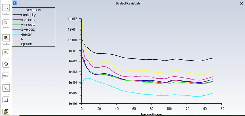
Residual Plot:

Temperature Contour:

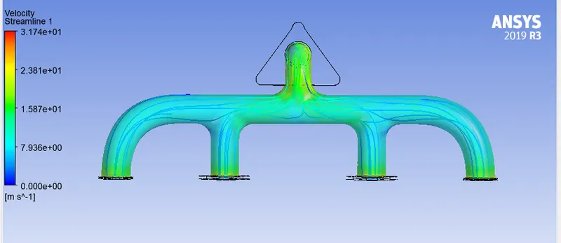
Velocity Steamlines:

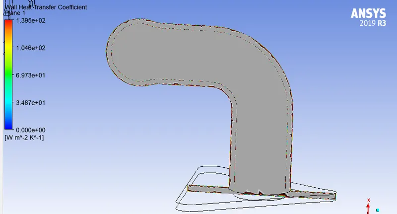
Wall Heat Transfer Coefficient:

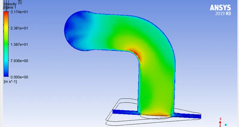
Velocity Plane:

Setup and Solution:

Case 2

V = 5 m/s

Temperature = 700 K

Heat transfer coefficient h = 20 W/m^2 K

K-epsilon

Realizable

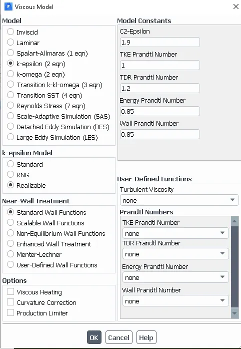
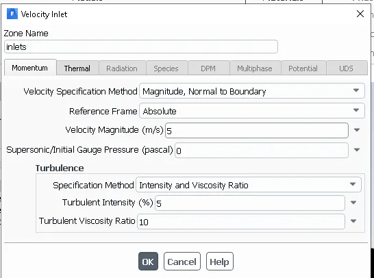
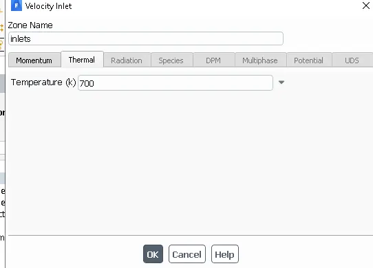
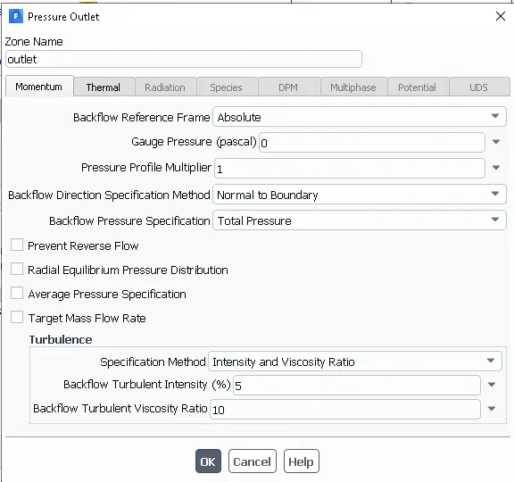
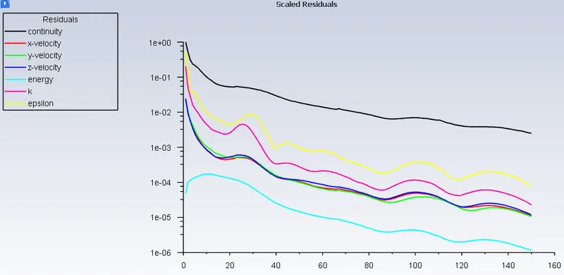
Residual Plot:

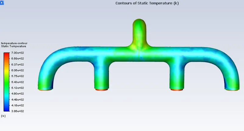
Temperature Contour:

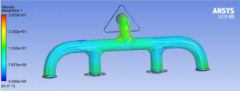
Velocity Steamlines:

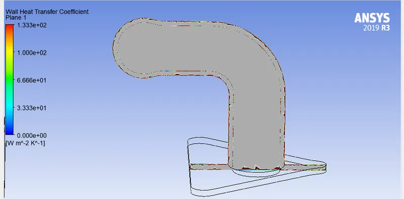
Wall Heat Transfer Coefficient:

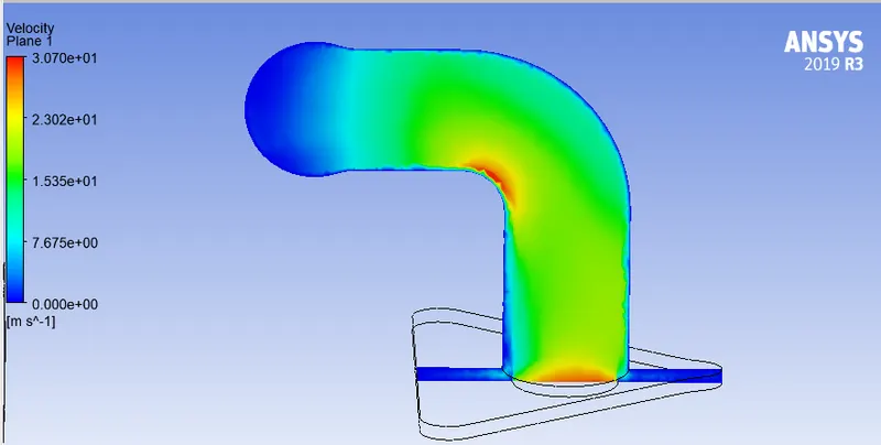
Velocity Plane:

Setup and Solution:

Case 3

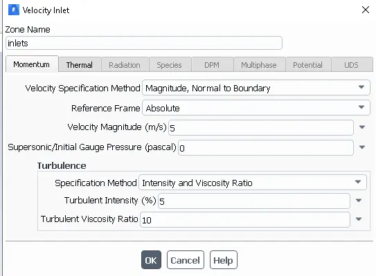
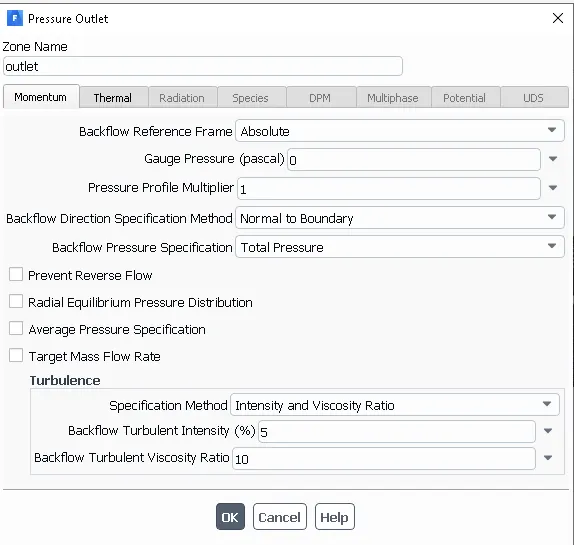
V = 5 m/s

Temperature = 700 K

Heat transfer coefficient h = 20 W/m^2 K

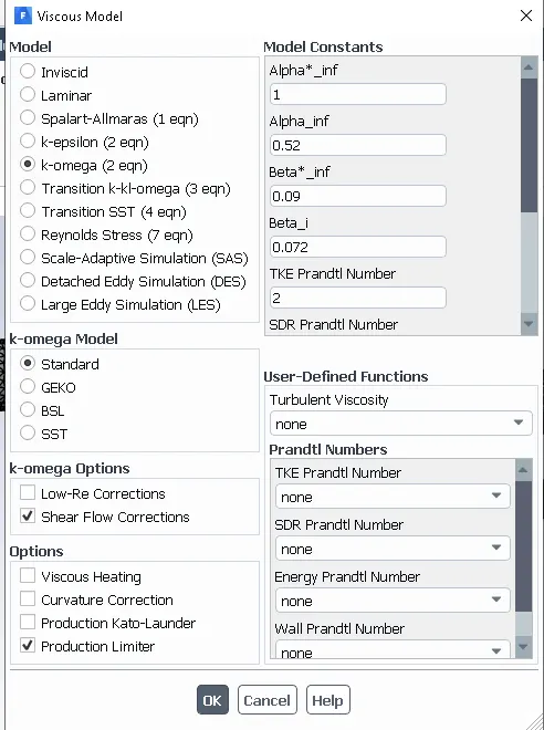
K-Omega

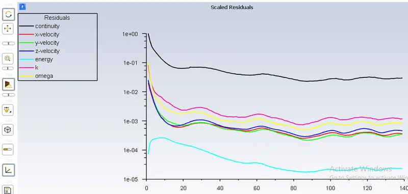
Residual Plot:

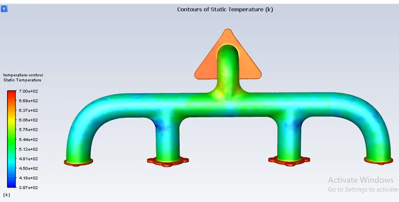
Temperature Contour:

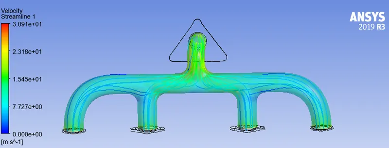
Velocity Steamlines:

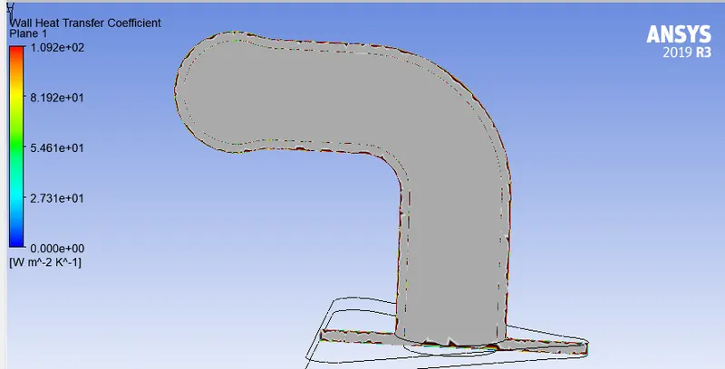
Wall Heat Transfer Coefficient:

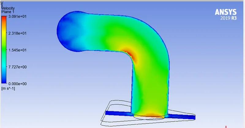
Velocity Plane:

K-epsilon Standard	Wall Covective heat transfer Coefficient	139 W/m^2 K
K -epsilon Realizable	Wall Covective heat transfer Coefficient	133 W/m^2 K
K-omega	Wall Covective heat transfer Coefficient	109 W/m^2 K

4. How would you verify if the HTC predictions from the simulations are right? On what factors does the accuracy of the prediction depend on?

The key to predicting the exhaust skin temperature requires a good understanding of the internal as well external fluid flow and heat transfer characteristics of the exhaust system. Experimental studies were performed by Malchow et al. (1979) in the straight section of an exhaust port of a four stroke spark ignition engine. Their objective was to construct an experimental set up to determine the heat flux from the exhaust gas to the wall for the straight portion of the exhaust port. Experiments were performed to investigate the timeaveraged heat transfer based on the effects of location in the exhaust and engine variables. 8 The data was correlated in the form of Nusselt-Reynolds number relationship for local and spatially averaged steady state heat transfer. The results revealed that the conventional steady state heat transfer relationships for developing flows underpredicts the heat transfer rates observed in the experiments. They found that, the deviation was mainly due to high frequency periodic flow and geometrical effects. Further, they developed an empirical correlation based on Nusselt-Reynolds relationship for the heat transfer rates based on the experiments. The constants in the correlating equation were found to be different for each of the four axial locations of measurement. The spatial averaged correlating equation is given as equation 2.1: 𝑁𝑢 = 0.0483 𝑅𝑒0.8 ∗ 𝑃𝑟1/3 (2.1) An augmentation factor was defined based on the ratio between the experienced Nusselt number and the ideal Nusselt number accounting for the effects due to engine induced pulsation. Temperature measurements were carried out by Wendland (1993) in the exhaust manifold, takedown pipes and post converter components. Wendland (1993) used both single and double walled pipes for the takedown portion of the exhaust along with several designs for the manifold. The measured Nusselt numbers were found to be always higher than that calculated for ideal flow with fully developed boundary layers similar to Malchow et al. 9 (1979). Wendland (1993) termed the ratio of a measured Nusselt number to the one from ideal flow correlation as Convective Augmentation Factor (CAF). Further, he found that the CAF is relatively constant across the range of engine loads and speeds tested. The Nusselt number correlation used by Wendland (1993) was based on the Sider-Tate (1936) relationship as given in equation 2.2: 𝑁𝑢 = 0.027𝑅𝑒0.8 ∗ 𝑃𝑟1/3 (2.2) The CAF values averaged over a component interior Reynolds number range of 4000- 20000 were 2.3, 3.0, and 1.6 for the manifold, takedown, and tailpipe respectively. It was also found that the percentage of the total external heat transfer from thermal radiation varied from 12%-18% for the tailpipe at low load to high load and 20-30% for the manifold. For the transient test cases Wendland (1993) applied steady state correlations to transient test. Instantaneous CAF values were calculated for the takedown and tailpipe and the equilibrium values were almost the same as in steady state testing. Wendland (1993) further suggested that the equilibrium CAF values could be used in modelling the performance of warmed up components.

Conclusion:

1. More finer the mesh more accurate result will be dispaly.

2. We kept the meshing values same for all three cases and study wall heat transfer values for k-epsilon-standard,k-epsilon-realizable,k-omega.

3. From these studies we realize that wall heat transfer values is highest for k-epsilon-standard and lowest for k-omega.

4. We successfully generate the result for all three cases.

References:

https://scholar.uwindsor.ca/cgi/viewcontent.cgi?article=8600&context=etd

https://convergecfd.com/benefits/conjugate-heat-transfer