Week 4 - CHT Analysis on Exhaust port

AIM:- To Perform CHT Analysis on Exhaust port.

OBJECTIVE:-

1. Give a brief description of why and where a CHT analysis is used.
2. Maintain the y+ value according to the turbulence model and justify the results.
3. Calculate the wall/surface heat transfer coefficient on the internal solid surface & show the velocity & temperature contours in appropriate areas.
4. How would you verify if the HTC predictions from the simulations are right? On what factors does the accuracy of the prediction depend on?

INTRODUCTION:-

• Conjugate Heat Transfer:-

1. Conjugate heat transfer (CHT) analysis can accurately predict heat transfer by simultaneous solving all the relevant solid and flow field heat transfer processes, for example: conduction through solids, free and forced convection in the gases/fluids and thermal radiation.
2. The CHT approach therefore has benefits for those applications where heat transfer is either non-uniform or difficult to calculate.

• Reynolds Number:- The Reynolds number is the ratio of inertial forces to viscous forces. The Reynolds number is a dimensionless number used to categorize the fluids systems in which the effect of viscosity is important in controlling the velocities or the flow pattern of a fluid.

`Re=(rho*V*D)/mu`

Where,

`rho=`Density of the fluid in`(kg)/m^3`

V= Velocity of the fluid in `m/sec`

D= Diameter of Pipe in m

`mu=` dynamic viscocity of fluid `(N*S)/m^2`

• Nusselt Number:- Nusselt number is the ratio of the Convective heat Transfer to Conductive Heat Transfer.

Nu=Convective Heat Transfer/ Conductive Heat Transfer

`Nu= h/((K/D)`

`Nu= (hD)/K`

Where,

h=heat transfer coefficient

D=Diameter of Manifold

K= Thermal Conductivity

• Prandtl Number:- Prandtl number is the ratio of the Momentum Diffusivity to Thermal Diffusivity.

Pr=Kinematic Viscocity/Thermal Diffusivity

`Pr=nu/alpha`

Where,

`nu=`Kinematic Viscocity

`alpha=K/(rho*cp)`

• Thermal Conductivity:- The thermal conductivity of a material is a measure of its ability to a particular material conduct heat.

`K = (Q*L)/ (A*ΔT)`

where

k is thermal conductivity (W/(m·K))

is specific heat capacity (J/(kg·K))

rho is density (kg/m3)

• Thermal Diffusivity:- Thermal diffusivity is the thermal conductivity divided by density and specific heat capacity at constant pressure. It measures the rate of transfer of heat of a material from the hot end to the cold end.

`alpha =(K)/(rho* c_p)`

• `Y^+`:-

To calculate the first layer thickness it is important to decide the desired Y+ value for the calculation, depending upon the turbulence layer theory or wall treatment method the requirement of Y+ value is varied accordingly. The first layer thickness is given as:

`ΔS=(Y^(+)⋅μ)/(U_(Freestreem)⋅ρ)`

GEOMETRY:-

Import geometry in Spaceclaim:

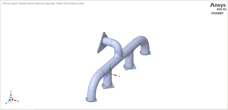
Then we have to check the Extra edges by using Repair >> Extra Edges

we have to perform the Volume Extract for make Separate Solid and Fluid, by using Prepair >> Volume Extract >> Apply.

we have to perform Share Topology For Making Combine nodes between Solid and Fluid Domain, by using Workbench >> Share >> Apply. after that we can get the Pink Edges we can confirm the Share Topology by it.

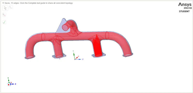
After that we get the Final Geometry as below:

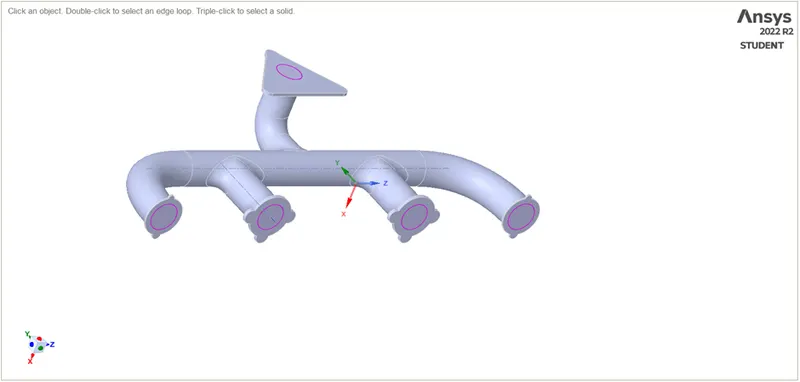
CASE-1

MESHING:-

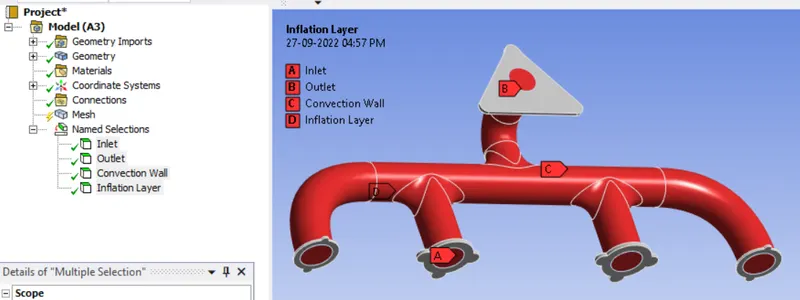
• Creating Named Selection:-

1. Inlet

2. Outlet

3. Convection Wall

4. Inflation Layer

• Base Mesh:-

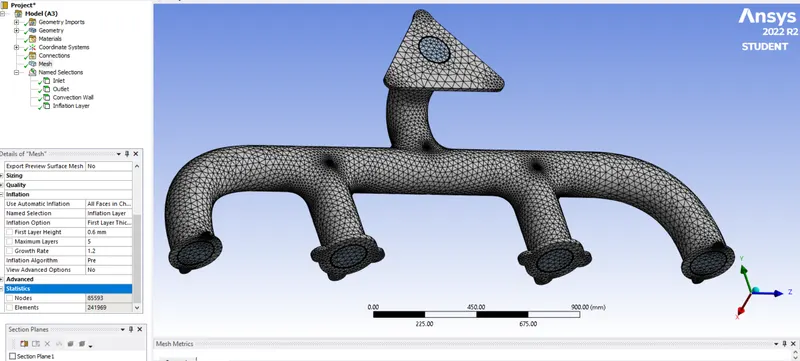
Here we used Default base Mesh (150 mm) For Meshing and also 5 layers & 0.6 mm First Layer Thickness is used for Inflation Layer. after that we are getting Mesh as below.

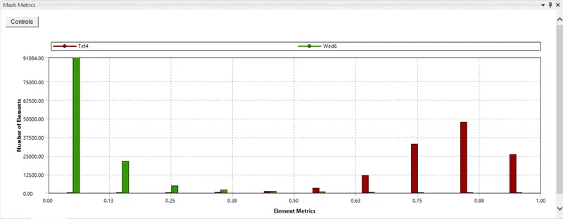
• Mesh Element Quality:-

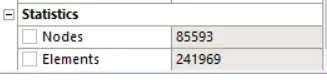
• Total No. of Elements:-

We are getting 241969 Total Elements for CASE-1

SOLVER:-

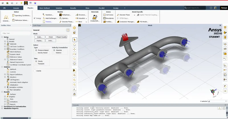
We are getting Interface as below

SET-UP:-

We are Using Set-up as below:

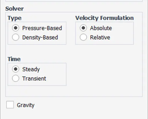
1	Solver	Pressure Based- Steady- Absolute
2	Energy	ON
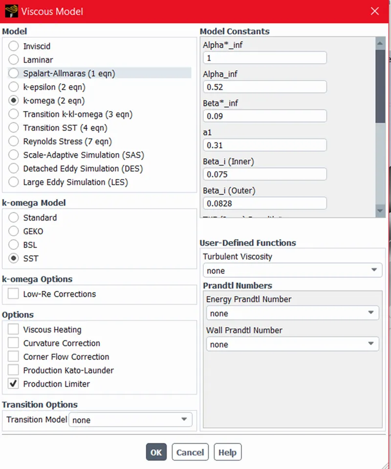
3	Viscous Model	K-Omega, SST
4	Cell Zones	1. Solid 2. Fluid
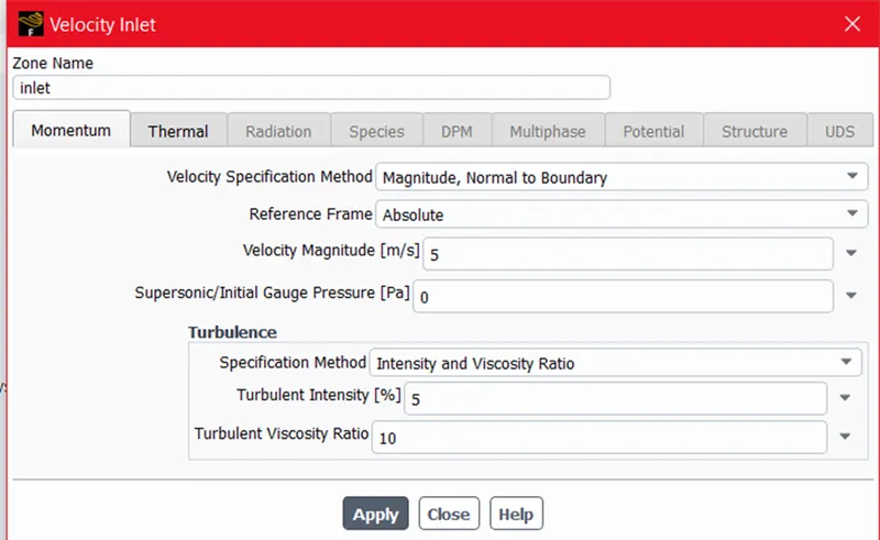
5	Boundaries	1.Inlet:- 5 m/s Velocity and 700 K Temperature 2.Outlet:- Standerd Pressure Outlet 3.Convection Wall:- 20 W/m^2K Heat Transfer Coefficient 4.Inflation Layer:- Fluid Volume

• Solver:-

Here We used Pressure Based Solver

• Viscous Model:-

Here We are using K-Omega SST Model, because we are Considering the Y plus as 10.

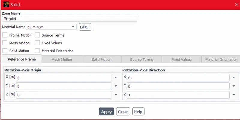
Now We have to Ensure the Solid Volume Should Have any Material, ain that case we used Aluminium as a Solid Material.

• Boundary Conditions:-

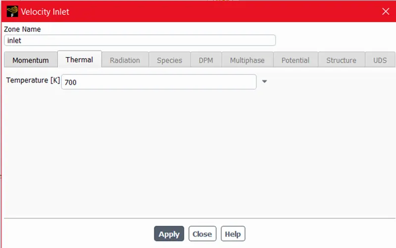
Velocity Inlet:-

We are Using Velocity Inlet as 5 m/s Velocity and 700 K Temperature.

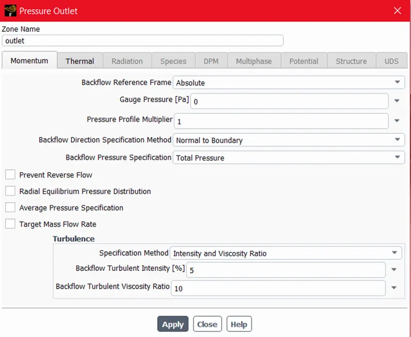
Pressure Outlet:-

Here we are Used Standerd Atmospheric Pressure Outlet.

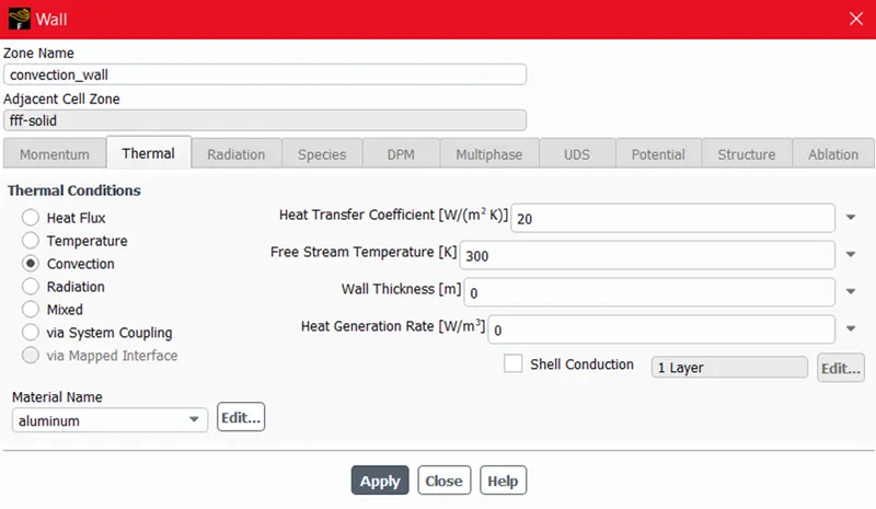
Convection Wall:-

Here we are Used Convection wall for Heat Transfer Coefficient as 20 `W/(m^2K)`

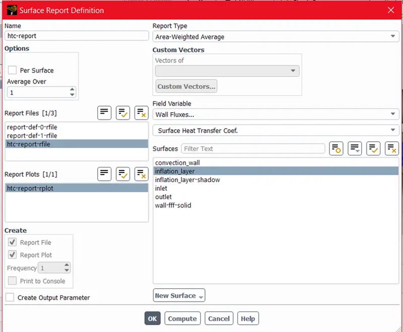
Then We Created the Report as Below.

1. Heat Transfer Coefficient Report.

2. Temperature Report.

3. Velocity Report.

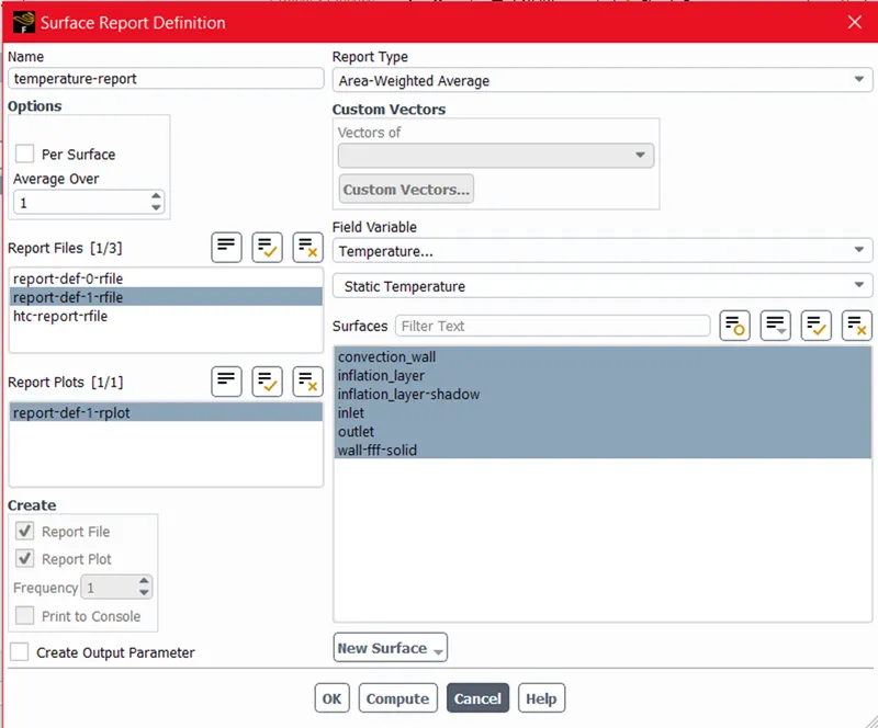
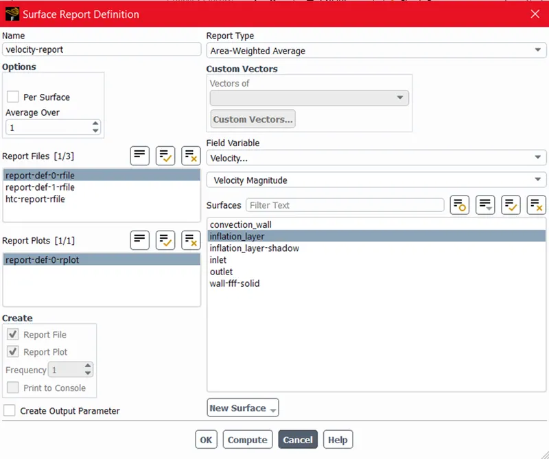
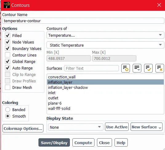
Then Initializes The solution by using Hybrid Initialization. Then we created Temperature and Velocity Contour as below.

Temperature Contour:-

Velocity Contour:-

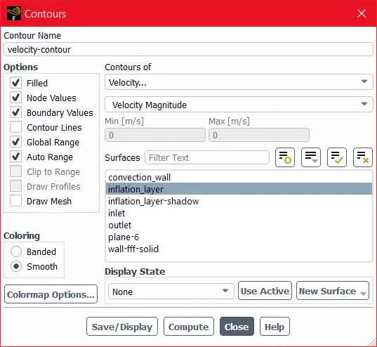
Then Run The Simulation For 150 Iterations.

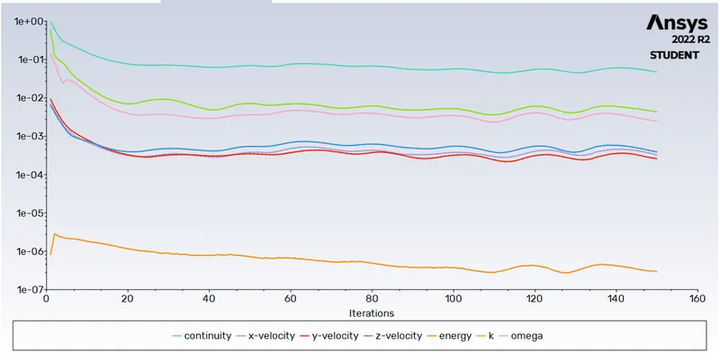
After Running Simulation We are getting Residual Plot, Velocity Plot, Temperature Plot and HTC Plot.

Residual Plot:-

Heat Transfer Coefficient Plot:-

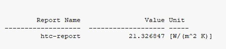
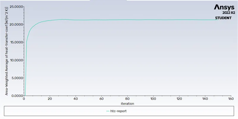
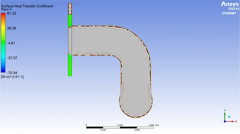
Here We are getting Heat Transfer Coefficent as 21.326847 W/m^2K.

Temperature Plot:-

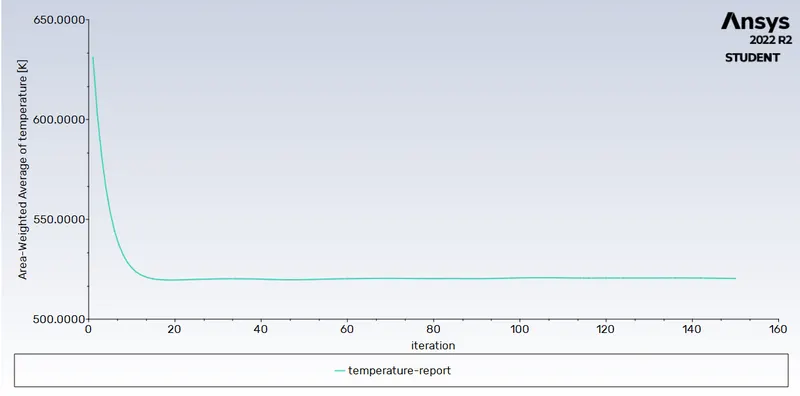
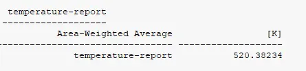
Here We are getting Average Temperature as 520.38234 K.

POST-PROCESSING:-

• Temperature Contour:-

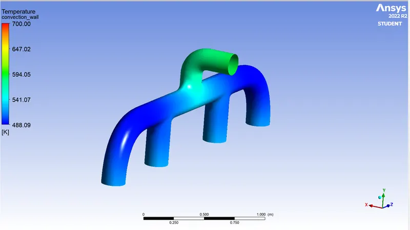
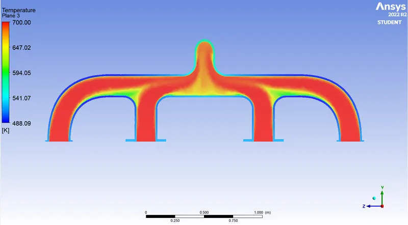
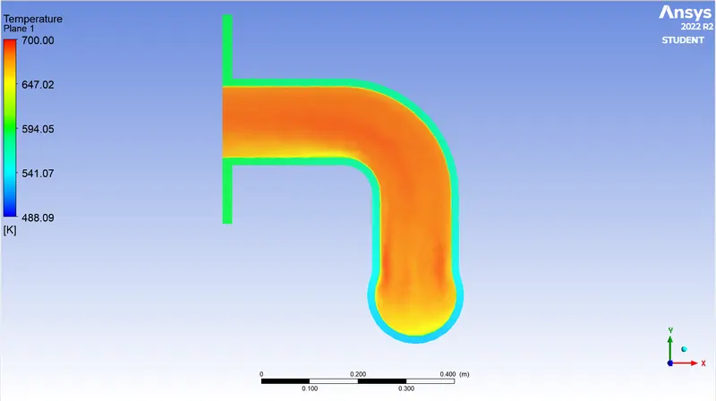
We are Getting Averege Temperature as 520.38234 K

• Velocity Contour:-

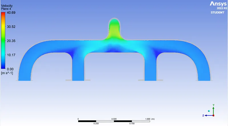
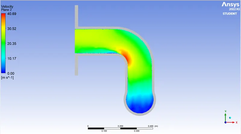
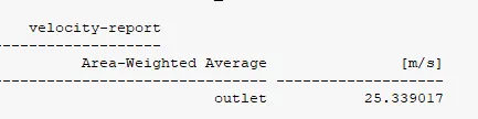
We are Getting Outlet Velocity as 25.339017 m/s

• Heat Transfer Coefficient Contour:-

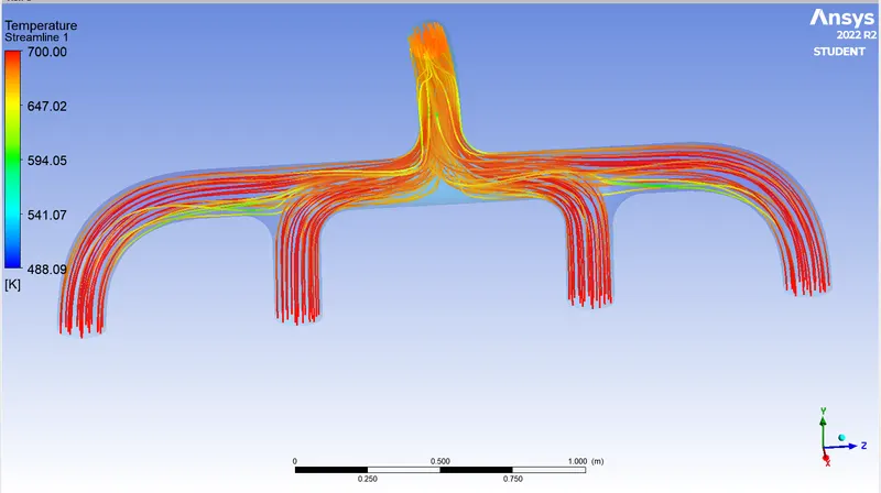
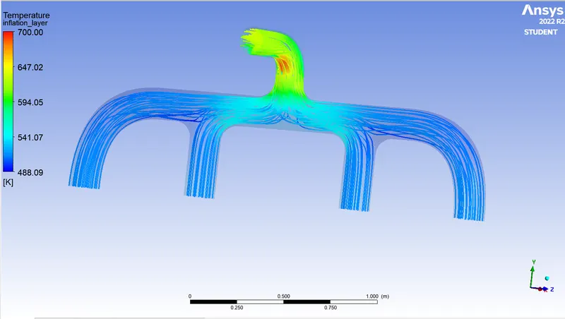
Streamline:-

• Temperature:

• Velocity:-

CASE-2

GEMETRY:-

Geometry is same as Case 1

MESHING:-

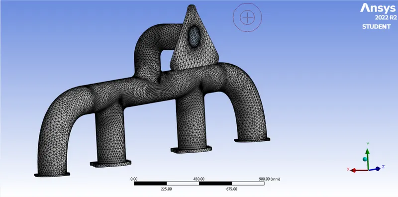
• Refined Mesh:-

Here we used Mesh(100 mm)For Base and also 5 layers & 0.6 mm First Layer Thickness is used for Inflation Layer. 10 mm Edge sizing for inflation layer ans 20 mm Face sizing for inflation layer. after that we are getting Mesh as below.

• Element Quality Criteria:-

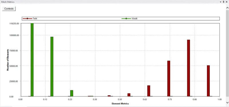
• Total Number of Elements:-

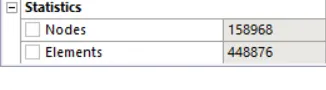
We are getting 448876 Total Number of Elements.

SOLVER:-

Solver Set-up same as Case 1

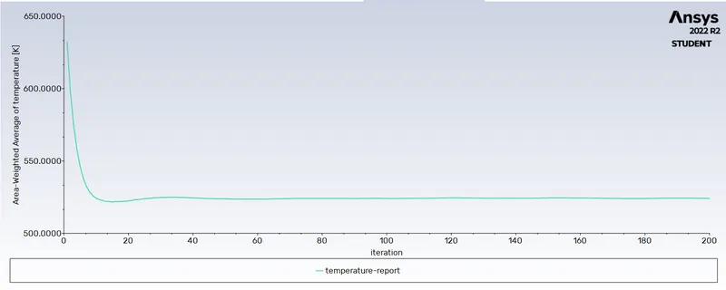
Then Run The Simulation For 200 Iterations.

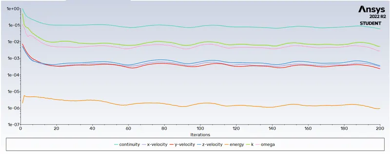
After Running Simulation We are getting Residual Plot, Velocity Plot, Temperature Plot and HTC Plot.

• Residual Plot:-

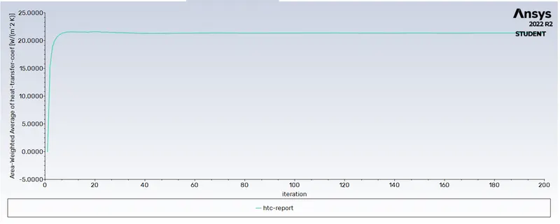
• Heat Transfer Coefficient Plot:-

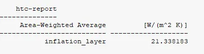
Here We are getting Heat Transfer Coefficent as 21.338183 W/m^2K.

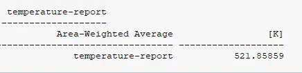
• Temperature Plot:-

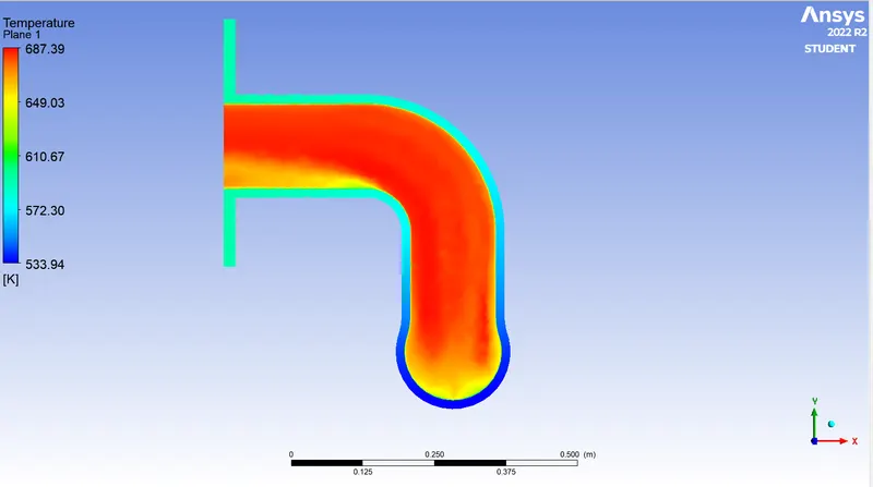
Here We are getting Average Temperature as 521.85859 K.

POST-PROCESSING:-

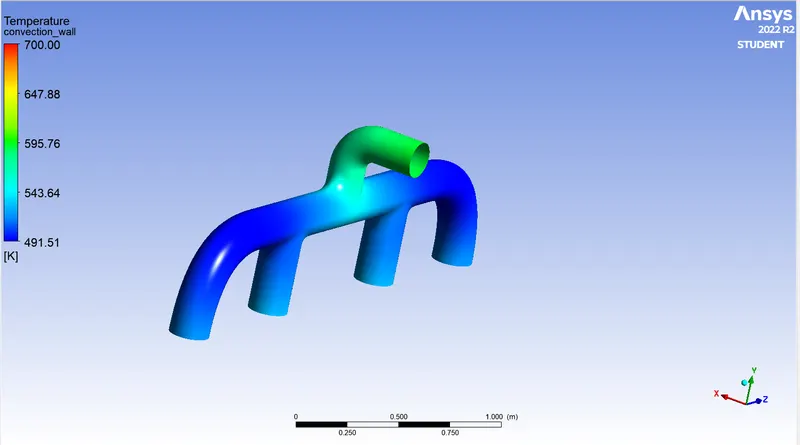
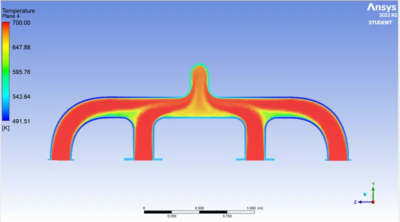
• Temperature Contour:-

• Velocity Contour:-

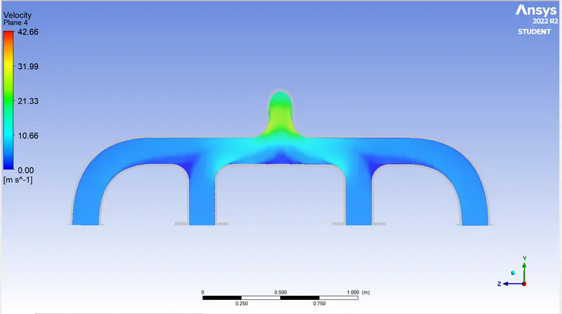
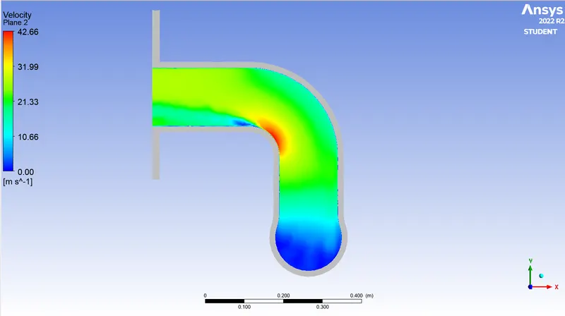
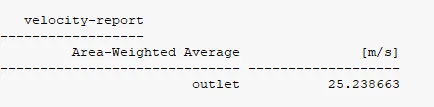
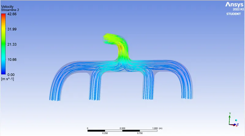
We are Getting Outlet Velocity as 25.238663 m/s

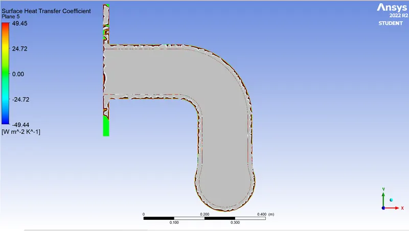
• Heat Transfer Coefficient Contour:-

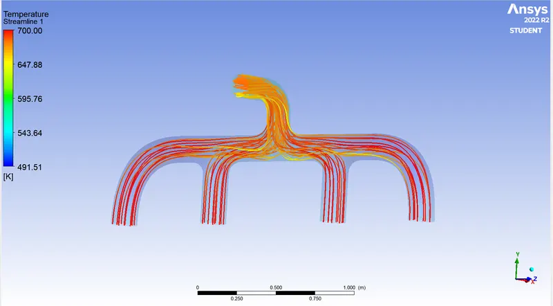
Streamline:-

• Temperature:

• Velocity:-

RESULT AND DISCUSSION:-

• Mesh Independence Study:-

Cases	Total Mesh Elements	Inflation Layer	Model	Heat Transfer Coefficient W/(m^2 K)	Average Temperature in K	Outlet Velocity in m/s
Case1 (Defualt Mesh)	241969	5 layers with 0.6 mm First Layer Thick	K-Omega, SST	21.326847	520.38234	25.339017
Case-2 (Refined Mesh)	448876	5 layers with 0.6 mm First Layer Thick	K-Omega, SST	21.338183	521.85859	25.238663
			Error w.r.t.Cases	1.13%	1.47%	0.40%

1. By observing above Table we can say that by Using Mesh element Size, Minute Diffrence Observed while Mesh Independence Study.
2. So we Observeed Case-1 is More prominent compared to Case-2 because Lesser Mesh Cells will Take Less Computational Time.

• Analytical Solution:-

First of all We are using equation as below.

`Nu= h/((K/D)`

`Nu= (hD)/K`---------------------(1)

Heat Transfer h= `(Nu*K)/D`

So, we need to find the Nu, K, D ( here we are concidering the dia as 0.168 m)

For Nu We use Dittus boelter equation.

`Nu=0.023*Re^0.8⋅Pr^n`--------------------(2)

Where n=0.4 for fluid being heated, Re

Prandtl number is given by ,

`Pr=(μ⋅Cp)/(K)`

Here `μ = 1.789 *10^(−5)` Cp=1006.43 J/kgK , K=0.0242 W/mk

putting all these value in equation we get,

`Pr=0.744`

Then `Re= (rho*V*D)/(mu)`

Re= 56833.

Put the Re and Pr in equation (2)

Then we get, Nu= 130.02.

Now put the all Values in equation (1)

Then we get,

h=18.95 `W/(m^ 2 ⋅ K)`

The Analytical Value of Heat transfer Coefficient is 18.95 `W/(m^ 2 ⋅ K)` and by Simulation is about 21.3268 `W/(m^ 2 ⋅ K)`.

We found 11% Difference between Analytical and Simulation Method.

CONCLUSION:-

• CHT Analysis on Exhaust port has been Done, by Using Ansys Fluent Software.
• Heat Transfer Coefficient, Temperature and Velocity Region has been Captured in Exhaust Port for the Simulation.
• By using Above Table We can Say that Case-1 is More prominent compared to Case-2 because Lesser Mesh Cells will Take Less Computational Time.
• we conclude the mass flow rate and Velocity is More at Outlet region.
• We conclude that Velocity is more at Elbow region of the Exhaust port.
• We observed The Heat Transfer Coefficient, Average Temperature and Outlet Velocity, is 21.326847 W/(m^2 K) , 520.38234 K and 25.339017 m/s Respectively.