Week 4 - CHT Analysis on Exhaust port

Aim: To perform Conjugate Heat transfer simulation in the ansys over a exhaust manifold using Ansys 21R1.

Introduction:

Conjugate in (CHT) suggests combined or coupled,This means analysis of heat transfer combining the heat transfer effects of solids and fluids present in the system.It is the study of conjugation of convection and conduction from solid and fluids.CHT analysis can precisely predict heat transfer by simultaneous solving all the relevant solid and flow field heat transfer processes.To simplify (CHT) analysis type allows for the simulation of heat transfer between solid and fluid domains by exchanging thermal energy at the interfaces between them.

The CHT approach therefore has benefits for those applications where heat transfer is either non-uniform or difficult to calculate empirically.the simulation of heat exchangers, cooling of electronic equipment, and general-purpose cooling and heating systems. for example: conduction through solids, free and forced convection in fluids and thermal radiation.

Need for the CHT Simulation

In the real world there will always be interaction between different states of materials like solid fluid, mostly the interaction will be related to temperature.So it is important to study how the heat flow varies with change of various parameters like the velocity of fluid,viscosity of fluid.

Study of CHT helps us to design efficient ways to dissipate or retain the heat from a body.For example In an automobile the engine has many parts that are in contact with the heat.Air convection is one way to cool the engine bay,other ways is using coolant jacket around the cylinders,the heat carried by the coolant are cooled by the natural forced convection of air from the fast moving car.There are many applications where heat dissipation is crucial for the efficiency.Like Ics,Computers etc.

Problem solving and modelling approach:

• Importing Ahmed body model into space claim
• Creating enclosures over the body
• check share topology is set to share
• click on the sharing in the workbench
• Perform Meshing
• pre processing (setting up the parameters and solvers,def for reports needed)
• Initialize and run fluent solver
• check for the convergence
• Post processing in the cfd post

Steps in the simulation setup:

Geometry

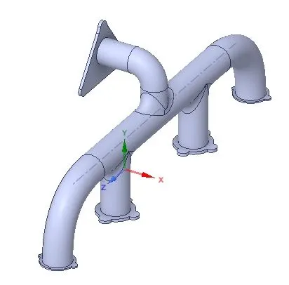
Geometry on which simulation is performed is imported into spaceclaim.

Extraction

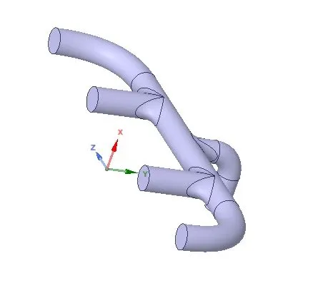
Fluid volume is extracted and the solid volume and fluid volume are moved to new components and the empty components are deleted.Share topology is set to share and in the workbench share is made between the solid volume and fluid volume for conformal meshing which helps in sharing the simulation information between them.

Fluid extraction

Solid Body

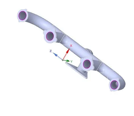
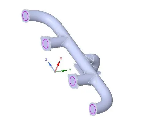
we need to make sure that shate topology is set to share.Then use the share tool in the workbench to share the topology between the fluid body and the solid body.To know whether the sharing is done we can see a pink circle on the exhaust ports.

Meshing:

Naming the exhaust manifold entities.

Insert body sizing and select the outer solid body and give the element size as 10mm.

Inflation layers:

Inflation layer is a body fitted mesh in which a mesh runs adjacent to the body.

Select the fluid volume and give the calculated inflation layer inputs.

Inflation layers are created in the exhaust manifold near the walls to capture the results more accurately and to visualize the variation of the required variables like heat transfer coefficient etc.

“Total Thickness” option in the Inflation settings is selected and maximum thickness of the boundary layer mesh is given.

Formula to calculate total thickness is `S_n=(a_1(r^n-1))/(r^n-1)`

r is the growth rate

The total thickness is 16

Mesh is generated.

Ansys Fluent

In the physics setup all the settings

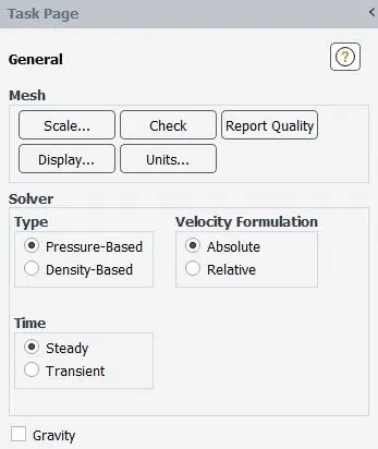
Pressure based solver is used

Energy is turned on as there is heat transfer taking place.

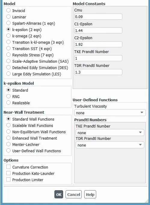
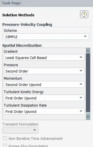
K-epsilon model is used as it is a turbulent flow

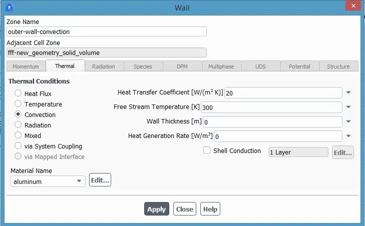
Convection is selected for outer wall

Create contours for heat transfer after initialization

Create a plane xy in the exhaust manifold

Plot definitions go to scaled

Results:

In the Cfd post processing we can visualize the Temperature,velocity steam lines and how temperature and velocity varies in the exhaust manifold at different locations.

Baseline Mesh:

element size 150mm

number of elements 137926

Mesh:

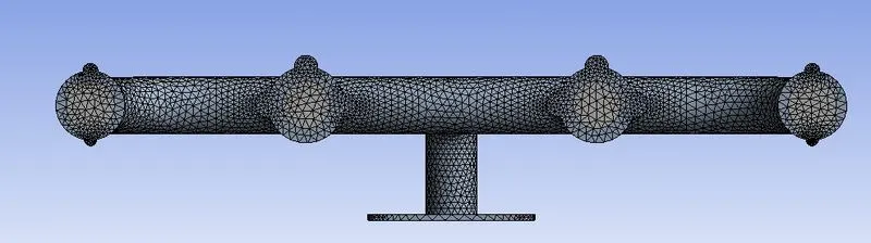
Residuals:

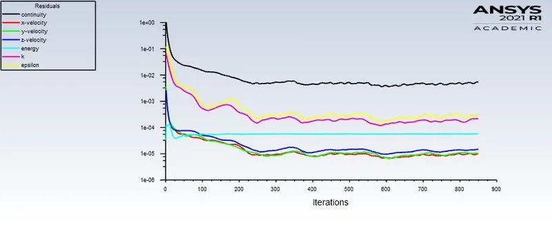
Temperature contour:

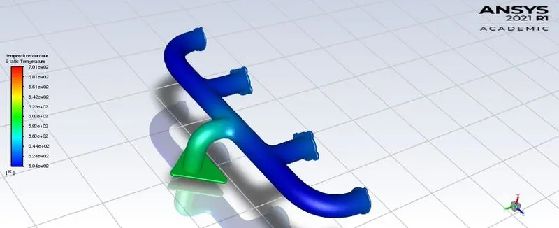
Velocity contour at the central xy plane :

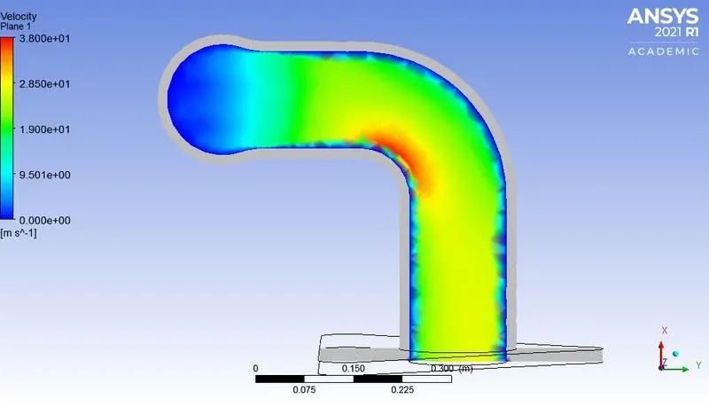
The baselinemesh shows the pixels so the variation of the velocity change is not smooth

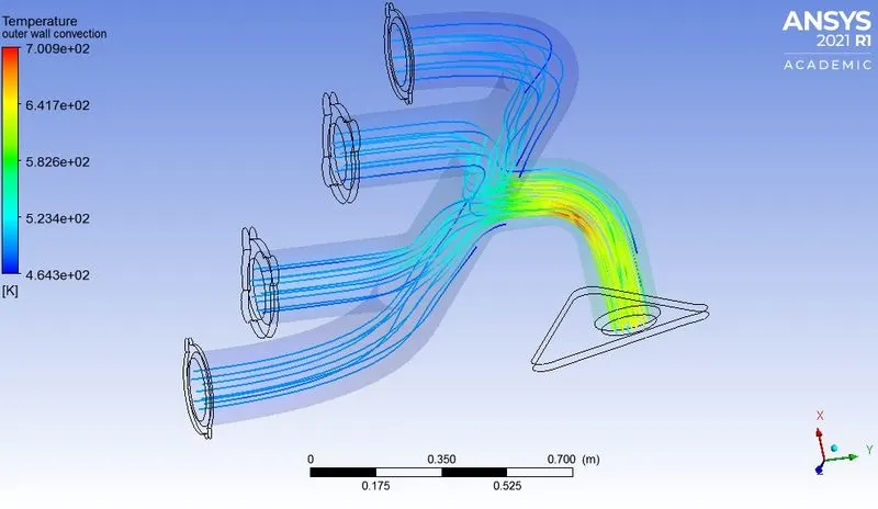
Velocity streamlines:

HTC

Increase in velocity increases turbulence, which in turn increases the effective thermal conductivity in the turbulent part of the boundary layer. ... Both these effects will increase the heat transfer coefficient when the fluid velocity increases

Heat transfer coefficient contour on the inner walls:

It is seen that the highest heat transfer coefficient is at the bend

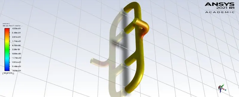
Max Heat transfer coefficient is 43.5 `W/(m^2k)`

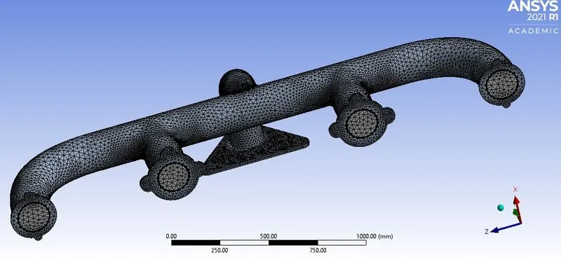
Case 2,Refined Mesh:

inner wall element size 150mm

outer wall element size 10mm

number of elements 371897

Mesh:

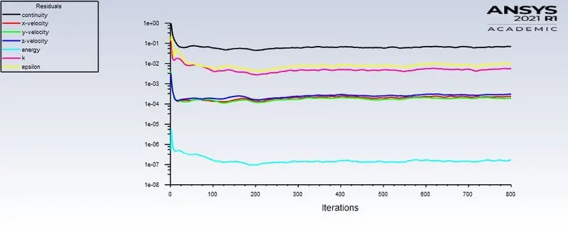
Residuals:

Temperature contour:

Velocity contour at the central xy plane :

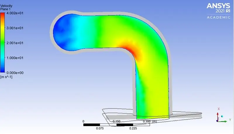
The refined mesh shows the smooth transition in the variation of the velocity change

Velocity streamlines:

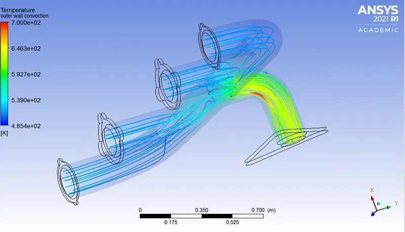
The red spot in the above two plots shows that the velocity is highest at the bent portion

Heat transfer coefficient on the inner surface:

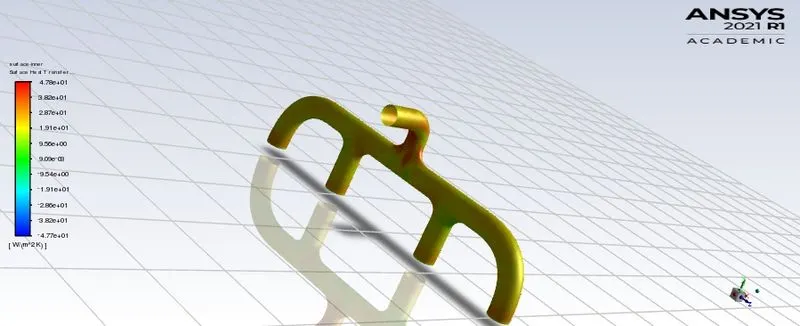
Max Heat transfer coefficient is 47.8 `W/(m^2k)`

Accuracy

The accuracy of the predictions depend upon the following factors

Mesh size majorly impacts the results of the simulation ,finer the mesh more accurate the results will be.But refining the mesh too much leads to increase in the computational time.It is better to refine mesh where needed.

Inserting inflation layers also affects the accuracy of predictions.We need to see that the inflation layers are not increasing the mesh size above half million cells which is not allowed for simulation.

Conclusion:

• The exhaust from 4 exhaust ports exit from one outlet,Due to mass conservation the velocity of the exhaust must increase at the bend of the outlet.
• This increase in velocity increeses the turbulence and thus increases the reynolds number resulting in the Increase of heat transfer rate there in the heat transfer coefficient increases at the bend.
• Baseline mesh takes less time to compute ,the refined mesh takes more time comparitively as the number of elements are increased.

Ways to verify if the HTC predictions from the simulations are right

• One way to know whether the HTC predictions are from the experimental data available.
• From numerical calculations we can calculate the heat transfer coefficient.After calculating nusselts number we can calculate the HTC 'h'.

nu = 0.023*(Re^(0.8))*Pr^n

Pr - prandtl number

Re - Reynolds number

`pr = nu/alpha=(mu/rho)/(k/(c_prho))=(c_p mu)/k`

From the prandtl number calculate the nusselts number

Re = `(rhoUL)/mu`

From the nusselts number we can find the Heat transfer coefficient 'h'

nu = `(hD)/k`