Week 4 - CHT Analysis on Exhaust port

CHT ANALYSIS

Introduction:

Conjugate heat transfer corresponds with the combination of heat transfer in solids and heat transfer in fluids. Conjugate heat transfer is observed in many situations. For example, heat sinks are optimized to combine heat transfer by conduction in the heat sink with the convection in the surrounding fluid. The Conjugate Heat Transfer (CHT) analysis type allows for the simulation of heat transfer between solid and fluid domains by exchanging thermal energy at the interfaces between them. Typical applications of this analysis type exist as, but are not limited to, the simulation of heat exchangers, cooling of electronic equipment, and general-purpose cooling and heating systems.

PROCEDURE

Baseline simulation:

GEOMETRY

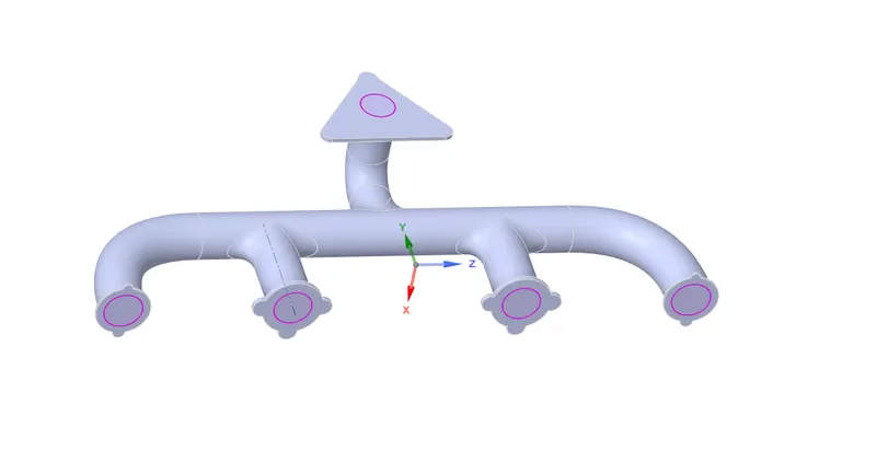
• In the space claim setup, we are setting up the CAD model geometry of the exhaust port which is already present in our system.
• Change the units to meters in the space claim and go to prepare Extract the volume by selecting the inner edges of the solid body.
• then go to repair remove the extra edges if any, and then go to the workbench and click on the share command and then enable the share topology.

The geometry of the Exhaust port is as below.

MESHING

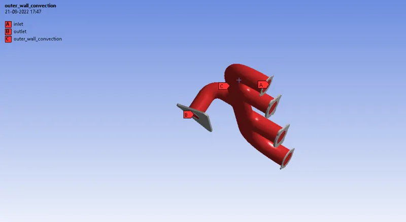
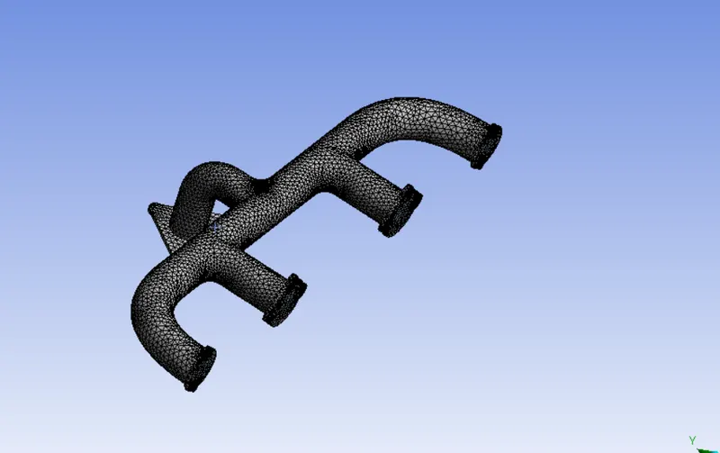
Since it is a baseline simulation, the default meshing that Ansys mesher does is checked. Named selections are provided to all the parts to apply boundary conditions when physics is set up. There are three named selections

(i) inlets, from where the hot exhaust gases enter the exhaust manifold

(ii) outlet, from where the exhaust gases leave

(iii) outer wall convection.

SETUP

• In the setup, we are setting up the physics of the simulation.
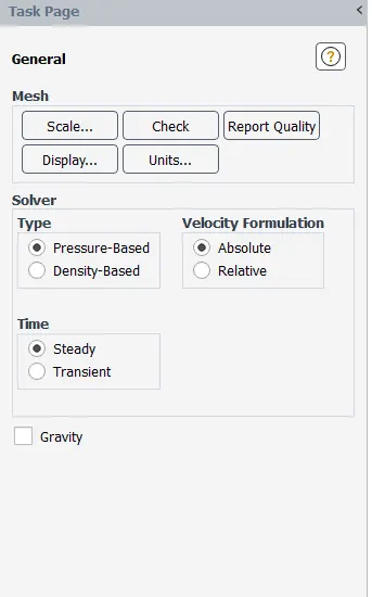
• Setup>physics>general setting>solver>type>pressure based.
• Setup>physics>general setting>time>steady.
• Setup>physics>general setting>velocity formulation > absolute

• physics>model>check energy.
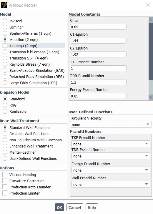
• physics>model>viscous model>K-epsilon

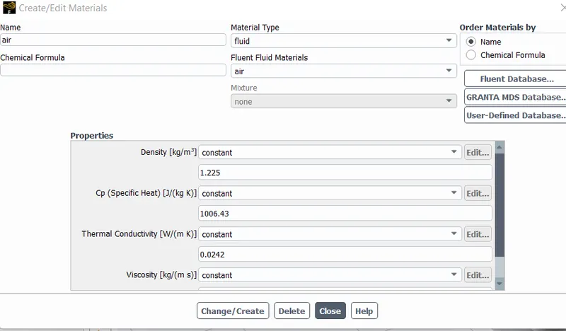
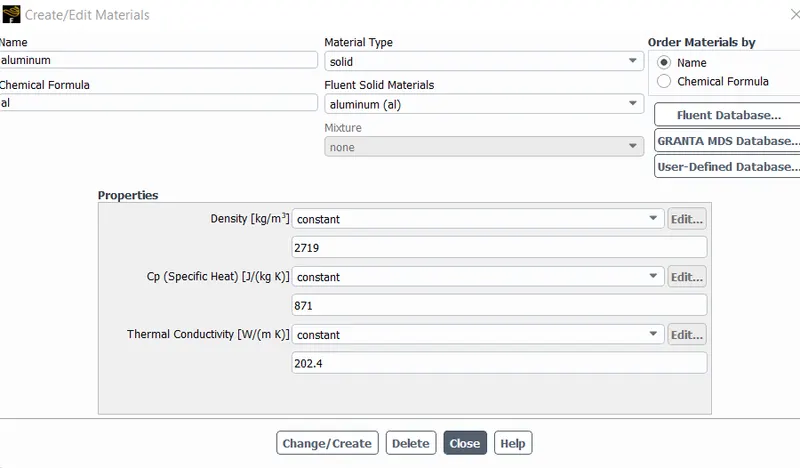
• physics> material>material type>fluid/solid.
• physics> material>fluent fluid material>air/aluminium.
• physics> material>properties> I have taken the default values here.

Boundary conditions

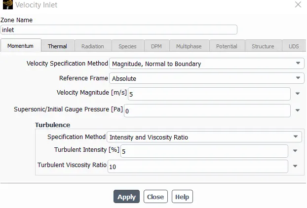
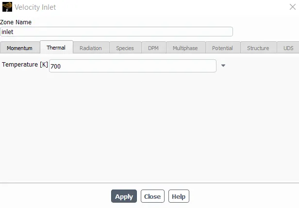
• Inlets: For the inlets, the velocity of the fluid inflow is taken as 5 m/s and the temperature of the fluid is taken as 700 K.

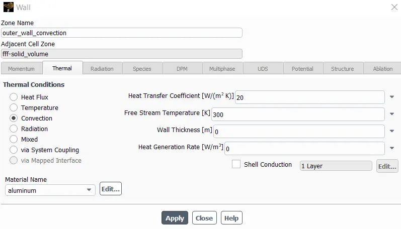
• The outer wall is considered a convection wall with a heat transfer coefficient of 20 w/`m^2 k` and free stream temperature as 300k.

v

• Outlet: Pressure boundary condition
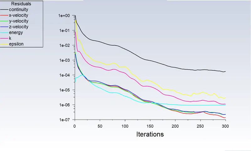
• Setup>solution>report>residuals>uncheck all the absolute convergence criteria and using the hybrid method initialize the simulation.
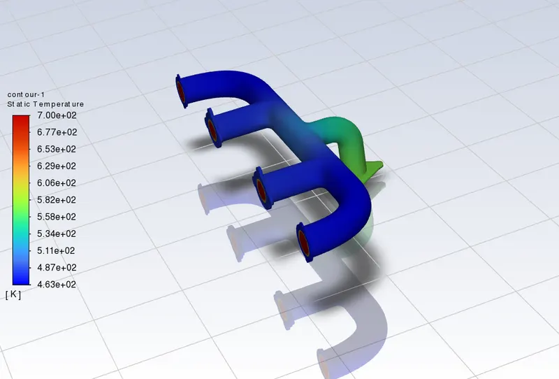
• create a temparature contour
• and run the simulation for 300 iterations.

Results:

Residuals plot:

Temperature contour:

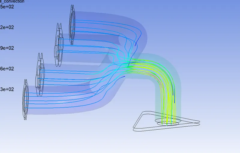
Velocity streamline contour

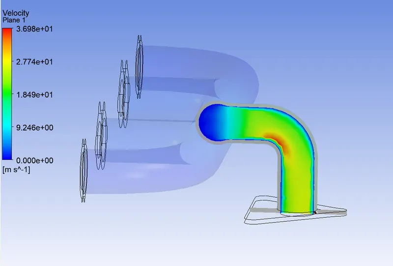
Velocity contour plane

• In current version of ansys parameters like surface heat transfer coefficient, surface nusselt number and some other parameters not available in cfd post, so to view such parameters in cfd post we have to export the results from fluent in .cdat format and we can import this in cfd post to view the results.

step1 :- file- export- solution data

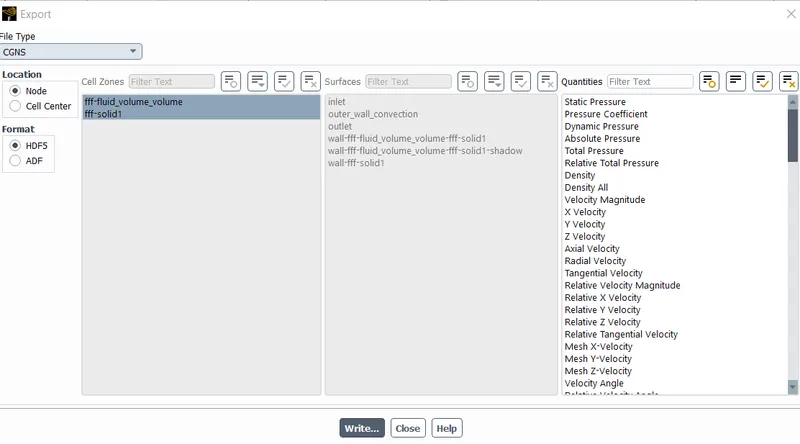
step2:- change the file type from cgns to .cdat for cfd post & ensight, and in the quantities select the required parameters make sure select all surfaces and zones

step3:- close fluent and open cfd post , go to file- load results

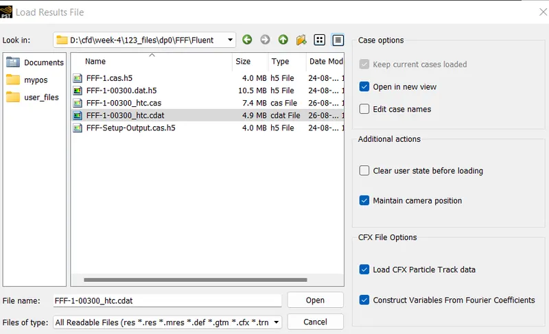
step4:- create a plane and plot required parameters

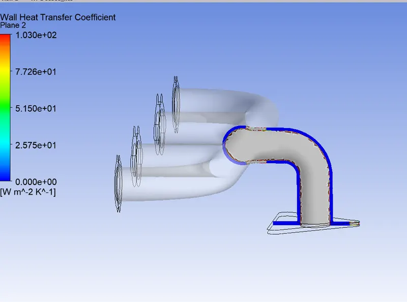
The baseline simulation gave coarse mesh results. Since the wall heat transfer coefficient is a wall phenomenon, wall modelling is required to capture the physics properly.