Week 4 - CHT Analysis on Exhaust port

* Description explaining why and where a CHT analysis is used.

* Maintaining the y+ value according to the turbulence model and justifying the results.

* Calculating the wall/surface heat transfer coefficient on the internal solid surface & the velocity & temperature contours are shown.

* Verifying if the HTC predictions from the simulations are right,and On what factors does the accuracy of the prediction depends.

Introduction:

CHT (Conjugate Heat Transfer) analysis is based on a mathematically structured problem, which describes the heat transfer between a body and a fluid flowing over or inside it as a result of interaction between two objects.

Conjugate heat transfer (CHT) simulations, which involve both fluid and solid domains within a CFD calculation, come with their own set of complications. This includes the solver's capability for handling and connecting thermal information between fluids and solids, as well as the workflow’s capacity to handle different thermal inertias.

The details are provided for temperature distribution and heat flux along the interface eliminating the need of calculating the heat transfer coefficient. Moreover, the heat transfer coefficient can be calculated later.

One of the simplest ways to realize conjugation is through numerical methods.

The boundary condition for the fluid as air and solid as aluminium is set and solved through iteration methods.

Application:

The conjugate heat transfer methods have become a more powerful tool for modeling and investigating natural phenomena and engineering systems in different areas ranging from aerospace and nuclear reactors to thermal goods treatment and food processing from the complex procedures in medicines to ocean thermal interaction in metrology.

CHT in recent years has significantly improved the cooling performance of electronic equipment such as the design of heat sinks and the design of heat exchangers for the waste treatment plant. One such application of CHT is the exhaust port system.

Solving and modeling approach:

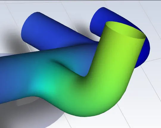
* The exhaust port was imported into the Spaceclaim.

* The exhaust port is a 3D model consist of four inlets and one outlet. Despite having isothermal boundary conditions and a uniform flow rate at the four inlets, the model cannot be cut into two halves to save computational time because of its asymmetrical nature. Therefore the whole model is discretized and is considered for meshing.

* CHT analysis requires both the solid and the liquid volume under consideration, Spaceclaim gives an option of volume extract for selecting edges for fluid volume.

* Both the solid volume and liquid volume are moved into one component.

* Spaceclaim gives an option for share topology, when share topology is selected and executed, the mesh from the fluid volume and the solid volume are said to be conformal with each other which is a requirement for CHT analysis.

* The exhaust port is loaded into the meshing window and then simulated for baseline mesh(K-epsilon) and the refined mesh(k-omega). (where y+ for K-epsilon is considered 50 and for K-omega y+ is assumed as 5)

* The named selections are created ( inlet, outlet, wall_heat_convective(fluid volume)).

* The necessary contour images and graphs are studied to understand the behavior of temperature, velocity, and surface heat transfer coefficient at the fluent interface.

Pre-processing and solver setting:

	Base Mesh	Refined Mesh
Number of elements	235715	367575
y+	50	5
Turbulence Model	K- epsilon	K-omega

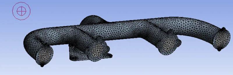
* y+ is calculated using y+ calculator which is available online . considering diameter of inlet as characteristic length

Fluent Setup:

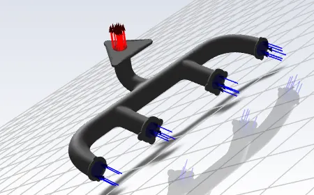
Boundary Conditions are,

Inlet :

Velocity inlet , velocity = 5 m/s , Temperature =700

Outlet :

Type - Pressure Outlet , Gauge pressure - 0 pa

Wall_heat_convective:

Type - wall , Thermal condition- convection Heat transfer coefficient - 20 `W/((m^2)K)`

The rest boundary condition values are set up as default values in ANSYS-FLUENT.

Energy equation is turned on , because in our simulation we are considering heat transfer .

Viscous model is set to k-epsilon(for base mesh) and k-omega(finer mesh).

Material properties

Material Name: Air (Fluid volume) & Aluminium(solid volume).

	Baseline Mesh	Refined Mesh
Residual plots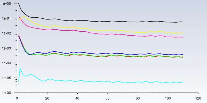
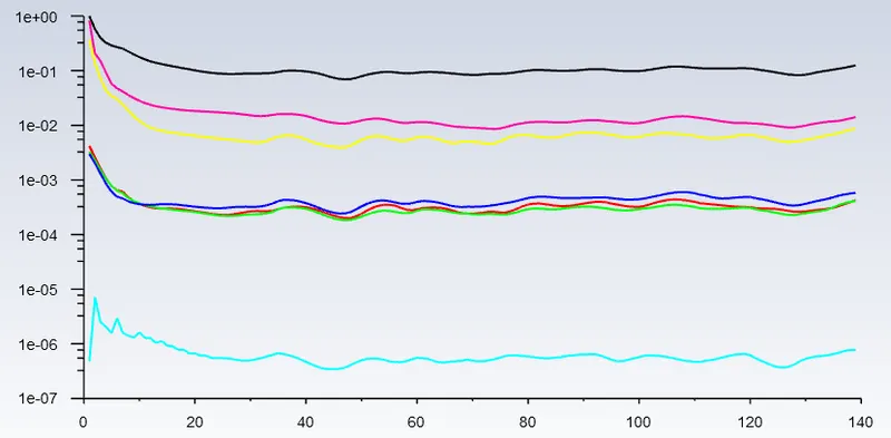Surface heat transfer coefficient on the internal solid surface
Temperature at Outlet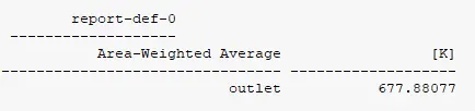
Velocity contour
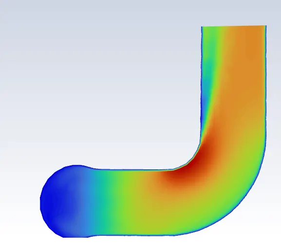
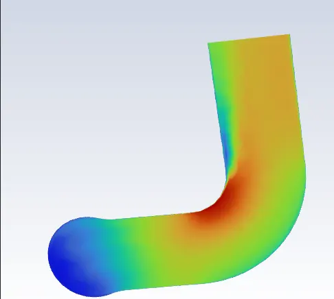
Temperature contour
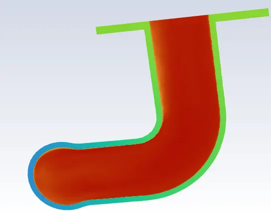
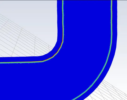
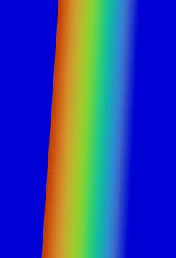
Wall Heat Transfer Coefficient	* Wall HTC is higher in the Bend , where velocity and temperature was higher. when velocity increases, it increases the viscosity which inturn increases heat.	*Note : Wall HTC is calculated near walls , here we have consideres Y+ as 5 , So figured is zoomed in to show wall HTC plot

Analytical solution

Convective heat transfer coefficient ,

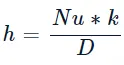
where Nu - nusselt number, k-thermal conductivity of a material(0.0242 W/mK)

The Reynolds number for the given flow is 58189 which suggests that the flow is turbulent in nature, the Dittus Boelter heat transfer coefficient relation can be used to determine the Nusselt number which is described mathematically as follows,

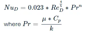
Cp is the specific heat capacity of the fluid = 1006.43 J/kgK

when calculated with default values Pr = 0.744

n is constant 0.3 heat transfer takes place from fluid to solid,

Therefore nusselt number = 136.48

Therefore convective heat transfer coefficient ,h = 19.4287 `W/((m^2)K)`

Conclusion

• The CHT analysis on the exhaust port was simulated successfully on ANSYS-FLUENT.
• The pressure-based, coupled scheme solver is used to discretize the whole geometry.
• The analytical value of the heat transfer coefficient is 19.4287 `W/((m^2)K)`
• The deviation of numerical heat transfer coefficient values from the analytical solution was found to be within 2% to 10%.
• The grid independence test was also observed during mesh refinement. The value of the heat transfer coefficient are close to each other. It is important that we limit ourselves to the refinement only to save the computational time and cost of the project.
  
• The value of the heat transfer coefficient is located in the cell adjacent to the wall which allows us to choose the value of Y+ = 5 (viscous sublayer) and the turbulent model K-omega SST.
• The presence of the boundary layer is quite visible near the inlet of the pipe where the viscous force makes the velocity near the wall to be zero causing a no-slip condition to occur, but as the flow is turbulent in nature (Reynolds number 58189.89)
• The velocity at the outlet is higher than the velocity at the inlet can be attributed to the presence of four inlets and one outlet.
• The accuracy of the heat transfer coefficient depends on selecting the suitable value of Y+ and turbulence model K-omega SST model. The heat transfer coefficient values predicted by CFD were validated against the numerical solution depicted the deviation in the range of 2-10%. However, the accuracy of K-omega SST model itself depends on the accuracy of the analytical solution, flow properties, and geometry.