Week 4 - CHT Analysis on Exhaust port

Week 4 - CHT Analysis on Exhaust port:

Aim & Objective:

• To perform a Conjugate Heat Transfer analysis and simulate flow inside an Exhaust port.
• To give a brief description about Conjugate Heat Transfer (CHT) analysis and where and why it is used.
• To perform CHT analysis on Exhaust Port.
• To select a proper turbulence model and maintain the correct Y plus value.
• To compute the Velocity, Temperature, Heat transfer coefficient contours and Y plus plots and other required contours and plots to show the results of the CHT analysis on the Exhaust Port.
• To validate the result and verify if the HTC predictions from the simulations are right or not.
• To state on what factors does the accuracy of the prediction depend on.

Introduction:

Exhaust manifold:

The exhaust manifold is tasked with collecting the exhaust fumes generated by an internal combustion engine and conveying them towards the catalytic converter or turbocharger. The name refers to the assorted inlets and outlets present on the manifold, which guide the exhaust fumes emitted from the cylinder head towards the underbody.

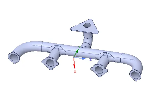
As the first component in the exhaust system, the exhaust manifold collects the exhaust fumes released from the engine cylinders and directs them to the catalytic converter. In turbocharged engines, the turbocharger is situated downstream of the exhaust manifold.

The design of the exhaust manifold has a significant influence on the performance and torque characteristics of an engine, as does the design of the connected pipes.

Conjugate Heat Transfer (CHT) Analysis:

The Conjugate Heat Transfer (CHT) analysis type allows for the simulation of heat transfer between solid and fluid domains by exchanging thermal energy at the interfaces between them. Typical applications of this analysis type exist as, but are not limited to, the simulation of heat exchangers, cooling of electronic equipment, and general-purpose cooling and heating systems. Efficiently combining heat transfer in fluids and solids is the key to designing effective coolers, heaters, or heat exchangers. The fluid usually plays the role of energy carrier on large distances. Forced convection is the most common way to achieve high heat transfer rate. In some applications, the performances are further improved by combining convection with phase change (for example liquid water to vapor phase change). Even so, solids are also needed, in particular to separate fluids in a heat exchanger so that fluids exchange energy without being mixed.

Heat Transfer in solids and fluids is combined in the majority of applications. As the solids are generally immersed in fluids the Conjugate Heat Transfer (CHT) analysis is very helpful in predicting the temperature distribution and heat transfer rates and their effects.

Conjugate Heat Transfer Applications:

Computational Fluid Dynamics (CFD) and more specifically conjugate heat transfer (CHT) analysis can accurately predict heat transfer by simultaneous solving all the relevant solid and flow field heat transfer processes, for example: conduction through solids, free and forced convection in the gases/fluids and thermal radiation.

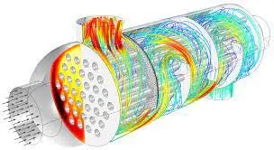
The conjugate heat transfer methods have become a more powerful tool for modelling and investigating nature phenomena and engineering systems in different areas ranging from aerospace and nuclear reactors to thermal goods treatment and food processing from the complex procedures in medicines to ocean thermal interaction in metrology. CHT in recent years has significantly improved the cooling performance of electronic equipment such as the design of heat sinks and the design of heat exchangers for the waste treatment plant. One such application of CHT is the exhaust port system.

Geeometry Dimension:

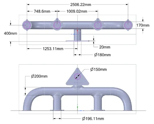
Geometry Setup:

• Open Ansys workbench and select the fluent setup in the project schematics.
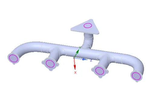
• open design modeler to prepare geometry for fluent CFD simulation and import the geometry of the Exhaust Port.
• Change the units to Meters.
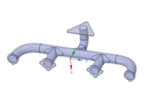
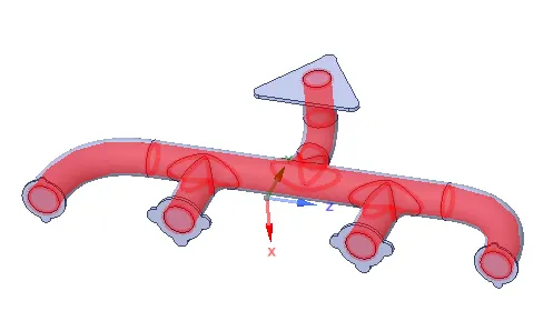
• Create fluid volume to represent the fluid flow by the following command. Prepare --> click on Volume Extract --> Activate edge selector and select all the open edges --> click on the green checkmark.

• By doing this we have two parts under the different components. In order to share geometry topology we need both parts in the same component. By selecting the both parts, select the ‘Move to the new component' option. By doing this, we have two empty components. To delete it, Right-click on the main geometry name and select ‘Delete Empty components’. Next, click on the new component, and in the topology option use share topology.

• To share geometry surfaces the following options are used. Workbench --> select ‘Share’.

Case 1:

Baseline mesh:

Model: K-epsilon

Mesh:

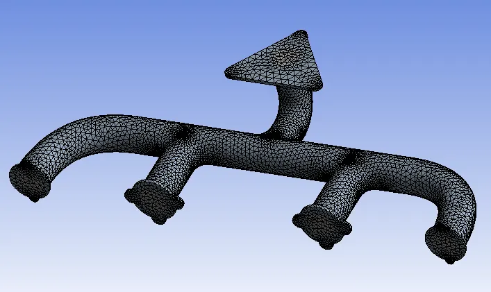
• In order to create a baseline mesh, click on 'Generate Mesh'.
• Create named selection. The named selections are as follows, Inlet, Outlet and Outer_Wall_Convection.

The baseline mesh is as follows:

Mesh Statistics:

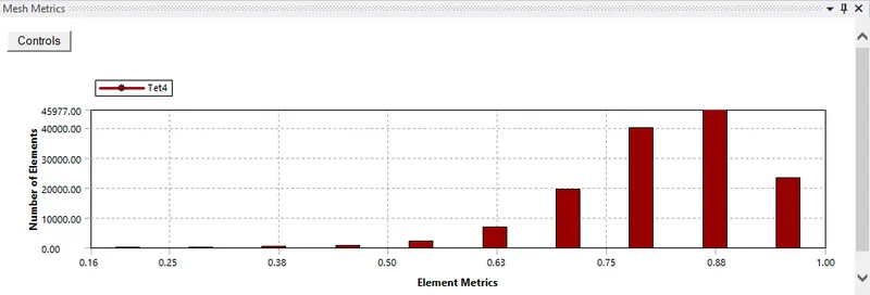
Mesh Quality:

Fluent Setup:

• Once the meshing part is completed, close the mesh and update the mesh.
• Open the "Setup". Set the Solver Type as Pressure Based and Absolute under Velocity formulation.
• Under Models enable the Energy equation and open Viscous select the k-epsilon model and click ok.
• Then under Material set the fluid to be air and solid to be Aluminum
• Under Cell Zone Conditions make sure that the selected fluid is air and the solid is aluminum.
• Select the Boundary Conditions parameter and set the boundary conditions for the created named selections.

Inlet:

Select the type to be velocity-inlet and assign the velocity. Set the temperature value of the fluid to be 700 K.

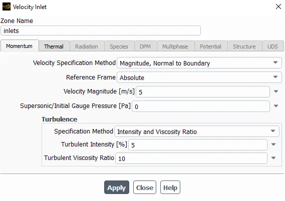
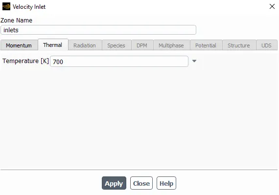
Outlet :

Pressure outlet: Gauge pressure = 0 pa

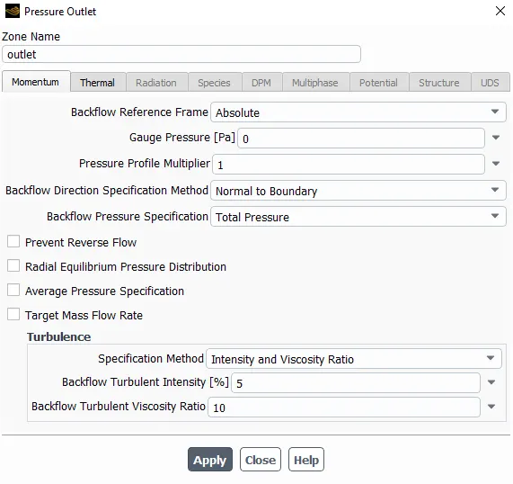
Outer_Wall_Convection:

We are checking convection in this problem so select convection and provide the Heat transfer coefficient as 20w/m²-K.

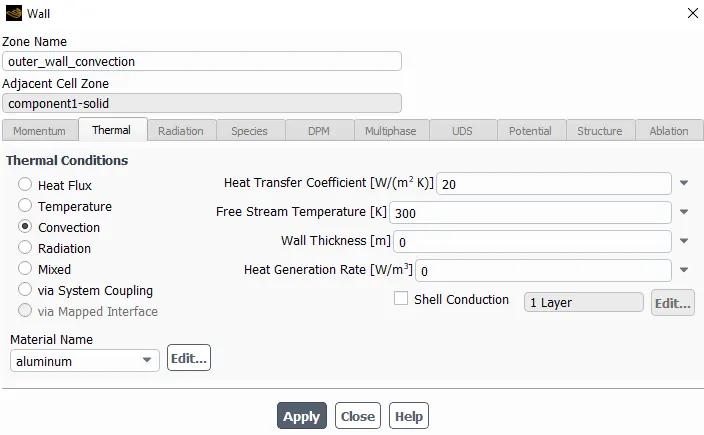
After completing the above steps "Hybrid Initialisation" is done.

Results From Baseline mesh:-

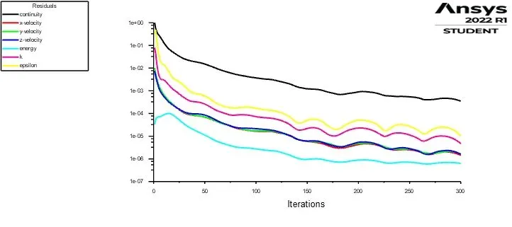
Residual Plot:

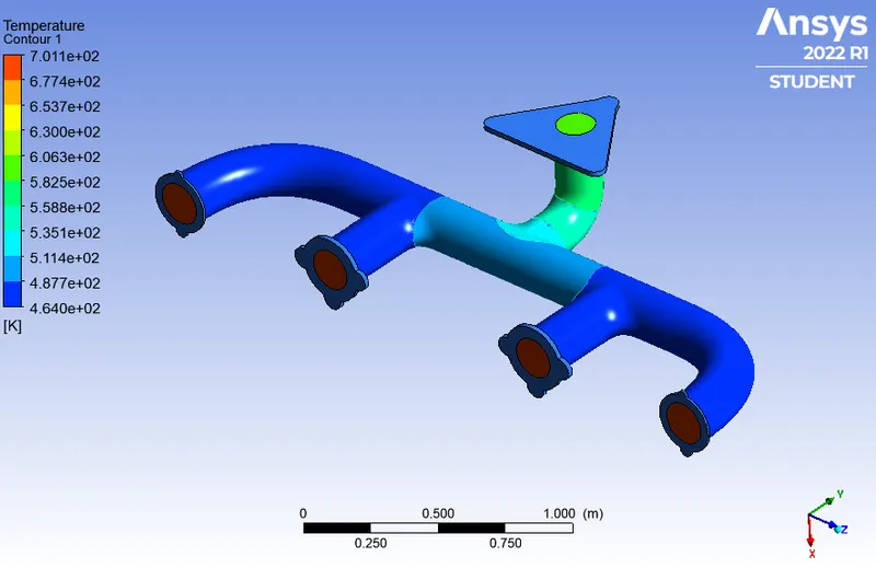
Temperature contour:

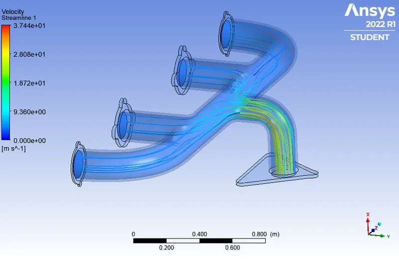
Velocity Streamline:

High-velocity region near the outlet:

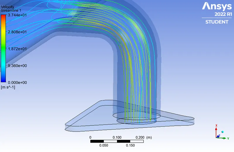
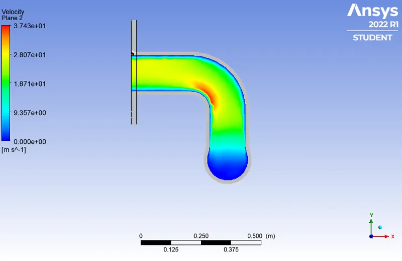
The above velocity contour plot predicts that the velocity is maximum at the bent area.

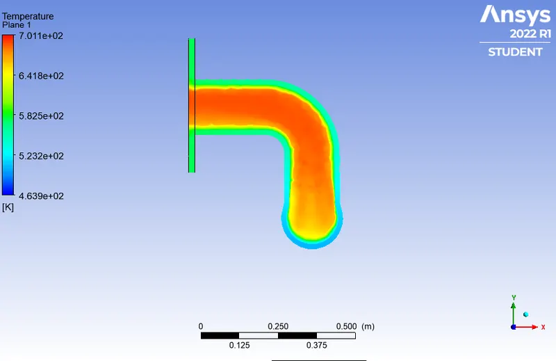
Temperature contour near the outlet:

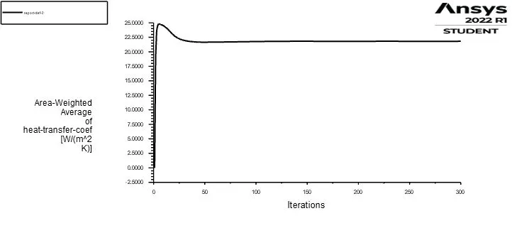
Surface heat transfer coefficient:

Wall Y+ Plot:

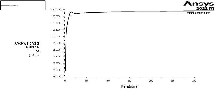
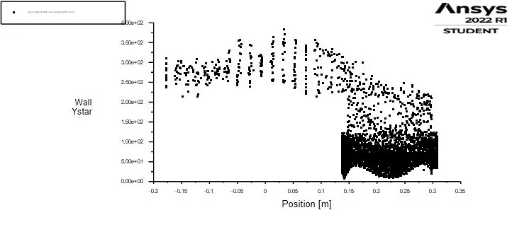
In the Y+ plot, we can notice the average Y+ value is 108 and exceeds upto 400. This value that we got from the baseline simulation is very high. This means it is not capturing the flow near-wall surface with proper effectiveness. Therefore, we need refined mesh with proper y+ plus value for our final mesh.

Surface heat transfer co-efficient value:

Case 2:

Refined Mesh:

Model: K-Omega SST

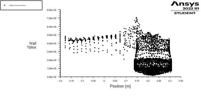
The y plus range should be in the range of 0-5 in order to calculate the First layer thickness.

Y-Plus value calculation:

Inlet diameter of the pipe 'D' = 0.17 m.

Density of air `rho` = 1.225 Kg/`m^3`.

Velocity of the fluid 'v' = 5 m/s.

Dynamic Viscosity `mu`= 1.7894*`10^(-5)` Kg/(m-s).

Reynolds Number = `(rho.v.d)/mu`

By substituting the above values we get,

Reynolds Number = 58190

`Y+ =(rho.U_T.Deltay_1)/(mu)`

Wall Shear Stress `T_w` = `(1/2).C_f.rho.V^2`

Skin Friction Co-efficient `C_f` = 0.079 * `Re^(-0.25)`(For internal flows)

`therefore`Skin Friction Co-efficient `C_f`= 0.0051

`therefore`Wall Shear Stress `T_w` = 0.07809375

Shear Velocity `U_T = root2((T/p)`

`therefore`Shear Velocity `U_T =0.2524`

`Deltay=(Y+*mu)/(rho*U_T)`

Case 2:

By considering the Y+ value as 40, we get the first layer thickness as the following value.

For the first layer thickness 0.00231495 m

Number of layers n = 5

Growth rate`Gr = 1.1`

Model: K-epsilon

Geometry Body sizing:

Outer body element size = 15 mm

Mesh:

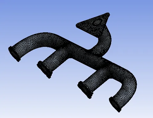
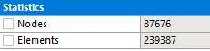
Mesh Statistics:

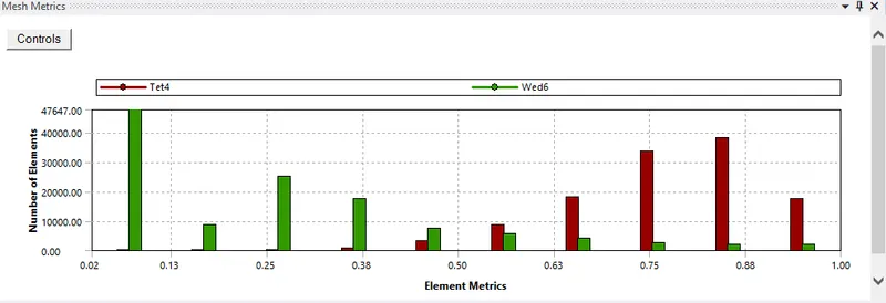
Mesh Quality:

The above mentioned steps for setting up the case is performed.

Results:-

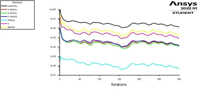
Residual Plot:

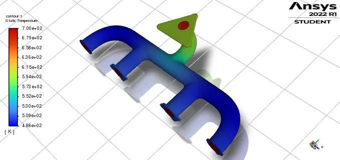
Temperature contour:

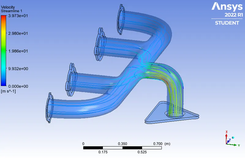
Velocity Streamline:

High-velocity region near the outlet:

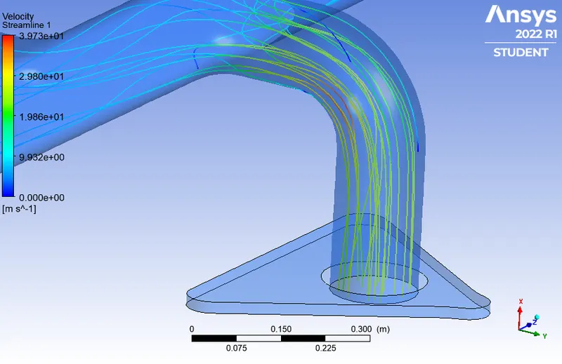
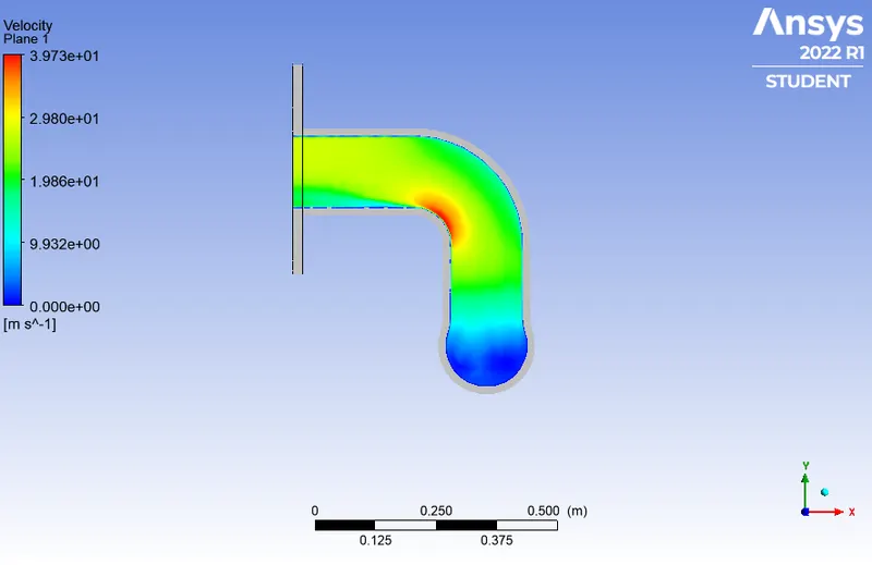
The above velocity contour plot predicts that the velocity is maximum at the bent area.

Temperature contour near the outlet:

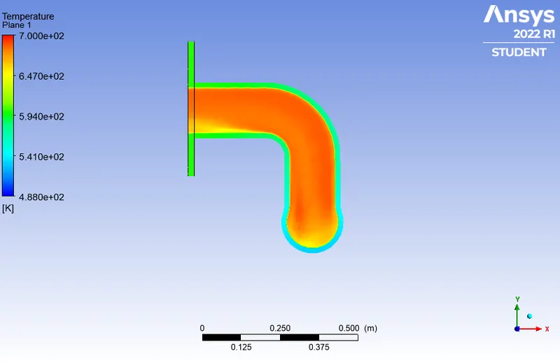
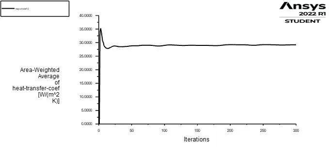
Wall Heat Transfer Co-efficient:

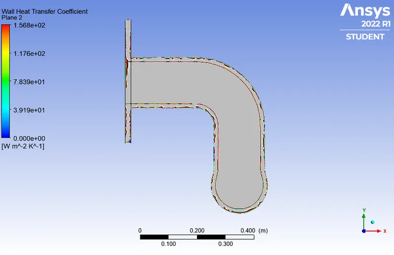
Surface heat transfer co-efficient value:

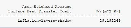
Surface heat transfer coefficient:

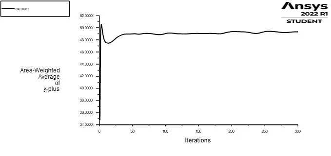
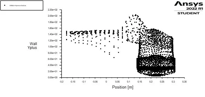
Wall Y+ Plot:

Case 3:

By considering the Y+ value as 1, we get the first layer thickness as the following value.

Number of layers n = 10

Growth rate`Gr = 1.2`

Model: K-omega SST

Geometry Body sizing:

Outer body element size = 15 mm

Mesh:

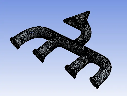
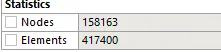
Mesh Statistics:

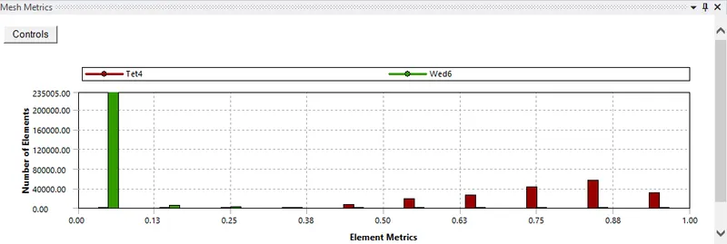
Mesh Quality:

The above mentioned steps for setting up the case is performed.

Results:-

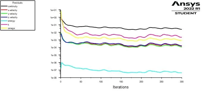
Residual Plot:

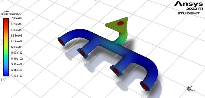
Temperature contour:

Velocity Streamline:

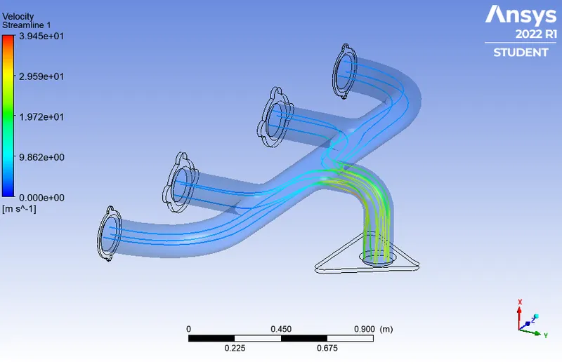
High-velocity region near the outlet:

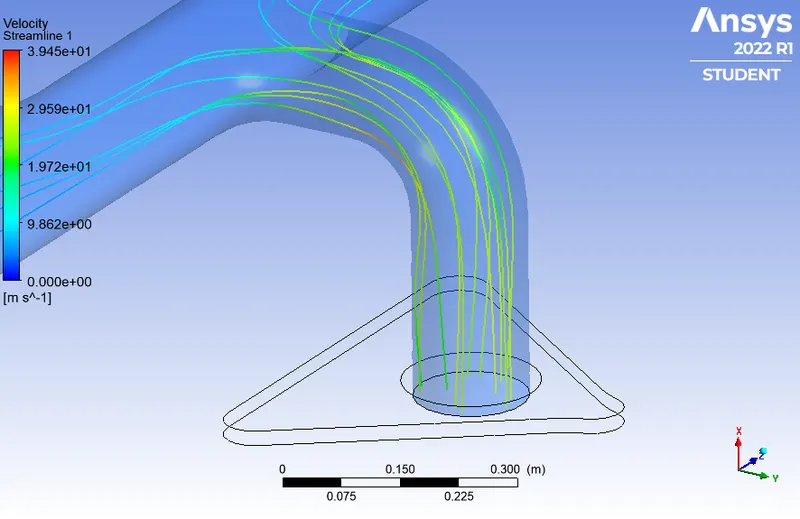
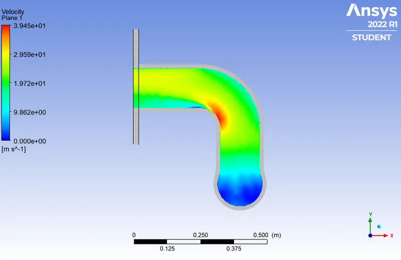
The above velocity contour plot predicts that the velocity is maximum at the bent area.

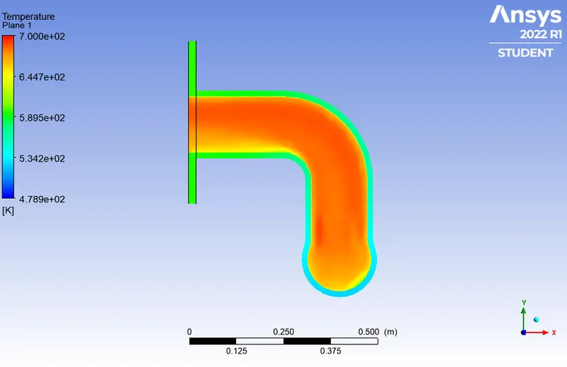
Temperature contour near the outlet:

Wall Heat Transfer Co-efficient:

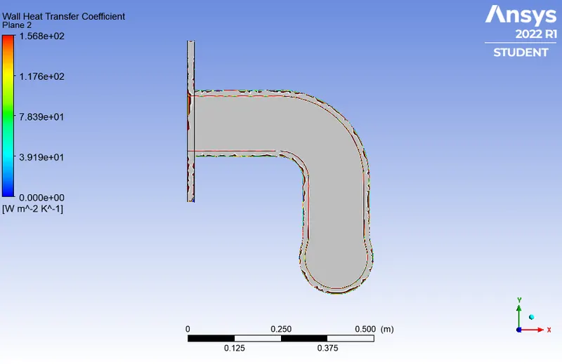
Surface heat transfer coefficient value:

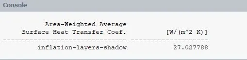
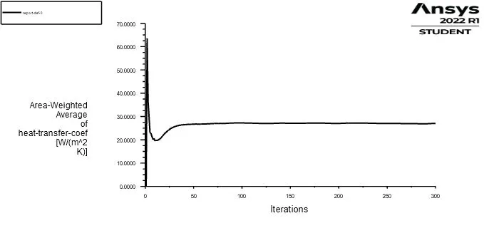
Surface heat transfer coefficient:

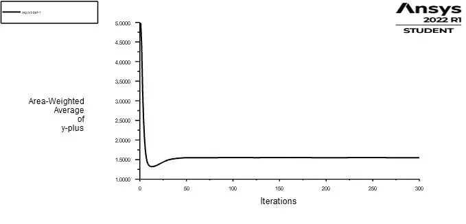
Wall Y+ Plot:

Analytical Heat Transfer Co-efficient Calculation:

At Inlet:

The heat transfer co-efficient can be calculated as, `h=(K/D_H)*N_u`

where,

K is the thermal conductivity of the liquid = 0.0242

`D_H`is the hydraulic diameter

`N_u`is the Nusselt number

`N_u=0.023*Re^0.8*P^(n)r`

n=0.3

`R_e`is the Reynolds number

`P_r` is the Prandtl number

Reynolds number = 5.8190e+04.

`P_r = (C_p.mu)/K` = 0.7949

`C_p`is the specific heat capacity of the fluid at constant pressure 1006.43 `J/(Kg.K)`

`N_u=0.023*(5.8190e+04)^0.8*(0.7949)^0.3`

`N_u=139.2182`

`therefore h=((0.00242/0.170)*139.2182) = 19.8181 W/(m^2.k)`

Conclusion :-

• The CHT analysis on the exhaust port was simulated successfully on ANSYS-FLUENT.
• The pressure-based, coupled scheme solver is used to discretize the whole geometry.
• The analytical value of the heat transfer coefficient is 19.81 `W/(m^2.K)`
• The deviation of numerical heat transfer coefficient values from the analytical solution was found to be within 5
  % to 10 % for the base line simulation and refined case.
• The presence of the boundary layer is quite visible near the inlet of the pipe where the viscous force makes the velocity near the wall to be zero causing a no-slip condition to occur., but as the flow is turbulent in nature (Reynolds number 58189.8960) the velocity profile goes from flat to the flutter and the boundary layer vanishes at the outlet.
• The velocity at the outlet is higher than the velocity at the inlet can be attributed to the presence of four inlets
  and one outlet. It satisfies the continuity geverning equation.
• The values predicted by the baseline mesh and the refined mesh were close to each other this can be attributed to the fact that the boundary keeps on growing and declining from the inlet to the outlet owing to change in velocity, thus the value is predominant at the outlet section of the exhaust port.