Week 4 - CHT Analysis on Exhaust port

Aim:

• Steady-state Conjugate heat transfer analysis on Exhaust port.

Description:

• Conjugate heat transfer analysis is based on a mathematically structured problem, which describes the heat transfer between a body and a fluid flowing over or inside it as a result of interaction between two objects. At the matching interface, the details are provided for temperature distribution and heat flux along the interface eliminating the need of calculating the heat transfer coefficient. Moreover, the heat transfer coefficient can be calculated later.
• One of the simplest ways to realize conjugation is through numerical methods. The boundary condition for the fluid and solid interface is set and solved through iteration methods. There are no right guesses for the values of the initial boundary condition for the convergence except through the hit and trial method.

Application:

• The conjugate heat transfer methods have become a more powerful tool for modeling and investigating nature phenomena and engineering systems in different areas ranging from aerospace and nuclear reactors to thermal goods treatment and food processing from the complex procedures in medicines to ocean thermal interaction in metrology.
• CHT in recent years has significantly improved the cooling performance of electronic equipment such as the design of heat sinks and the design of heat exchangers for the waste treatment plant. One such application of CHT is the exhaust port system.

Why CHT :

• Understanding of the complex heat transfer mechanisms and the interactions between those mechanisms to improve the performance and increase the lifespan of the components to be analysed.
• Conjugate Heat Transfer analysis provides the temperature distribution in solid and fluids, and clear insight on velocity distribution and mechanism of heat transfer of fluid, like in engines.
  It is more accurate and fast to simulate the problem.
• Can be used in complex scenarios like in automotive components or in power plant components.
• Multiple number of regions can be simulated.
• All types of region combination can be simulated like solid-fluid,fluid-fluid, etc.

Where is CHT analysis done :

• Analysis of Heat transfer mechanism in turbocharger.
• HVAC systems.
• Burners, combusters, electronic devices.
• Automotive, power plants and various other applications.
• Heat transfer in ribbed passages.
• Heat transfer in micro-channels.
• Heat transfer in fin arrays.
• Heat transfer in mobile phones.
• Drying of a porous flat plate.

Procedure:

• Open Ansys workbench and drag the Fluid Flow(Fluent) to main window.

• Click on geometry to import the geometry file.

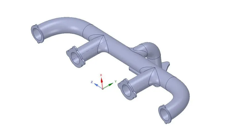
• Select the edges of the surface which the fluid flow takes place by using Volume Ectract option in geometry window.

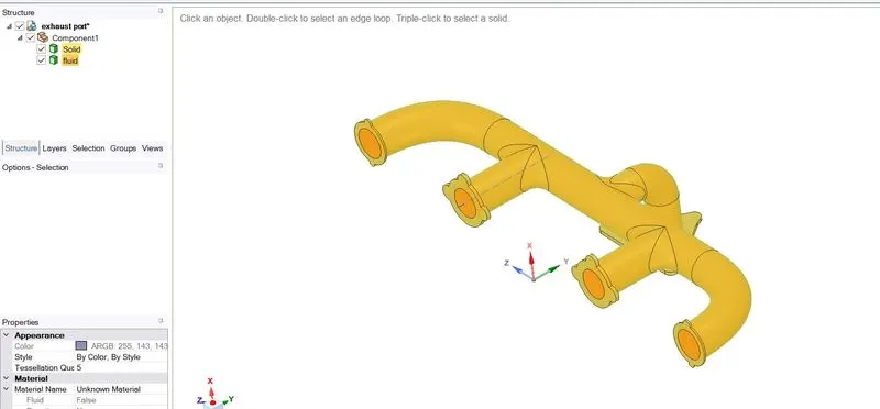
• Then update geometry in main window. After that click mesh.
• Select the faces by using selecting face option then name the faces like “Inlet, Outlet,outer-Wall-convction,inflation-layer”.

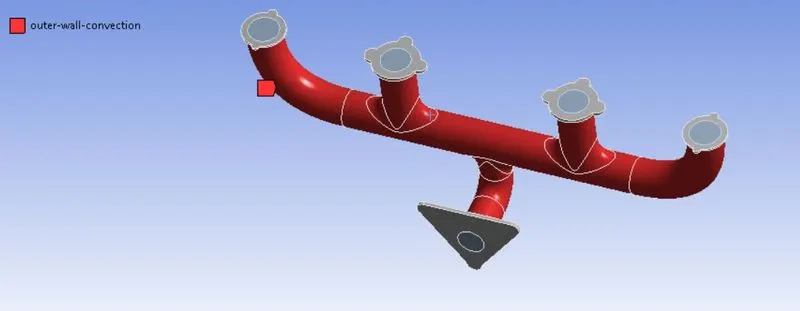
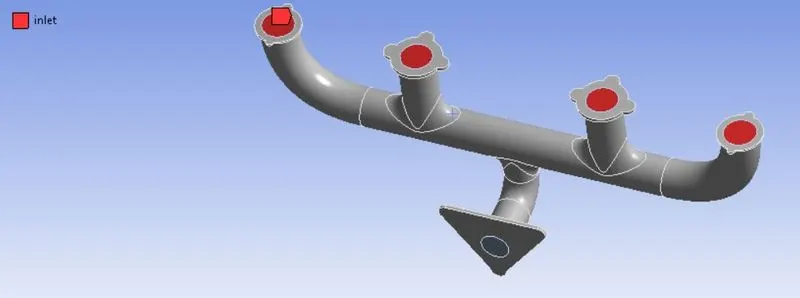
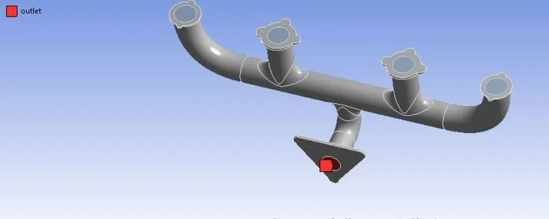
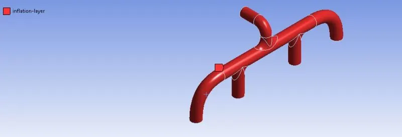
• Go to mesh enter mesh size as 90mm and the max size also 100 mm, insert sizing mesh select the outer-wall-convection enter the element size as 10 mm, select the named selection select inlet in exhaust port enter mesh size as 5mm then generate the mesh for the first refined smulation.

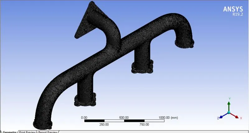
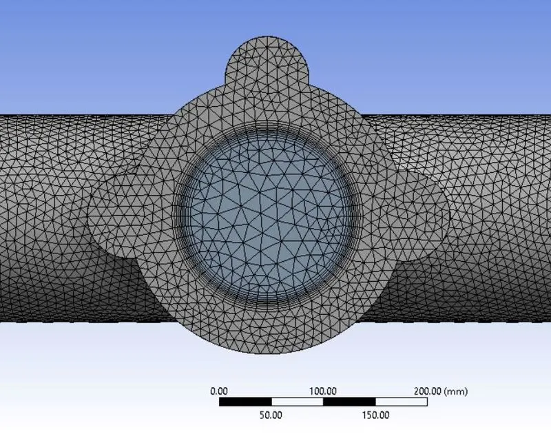
• For second and third refinement change the mesh size as 80 and 70 respectively. After the meshing update the mesh in main window then go to the setup option.
• After loading the geometry in graphics window change the appropriate units. Then check the mesh.
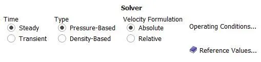
• Select k-epsilon,Steady-state, the pressure-based solver model to solve. Then select the fluid material as air and solid material as aluminium. After that enter the boundary condition such as inlet velocity, temperature, heat transfer coefficient and pressure. Then initialize the solution and enter the no. of iteration then click calculate to run the simulation.

• Create a heat transfer coefficient plot for each iteraion. Run the simulation.
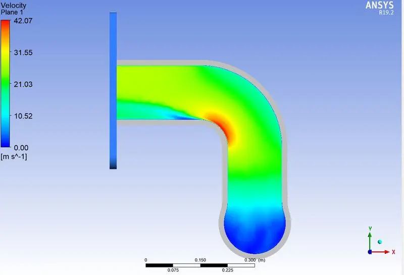
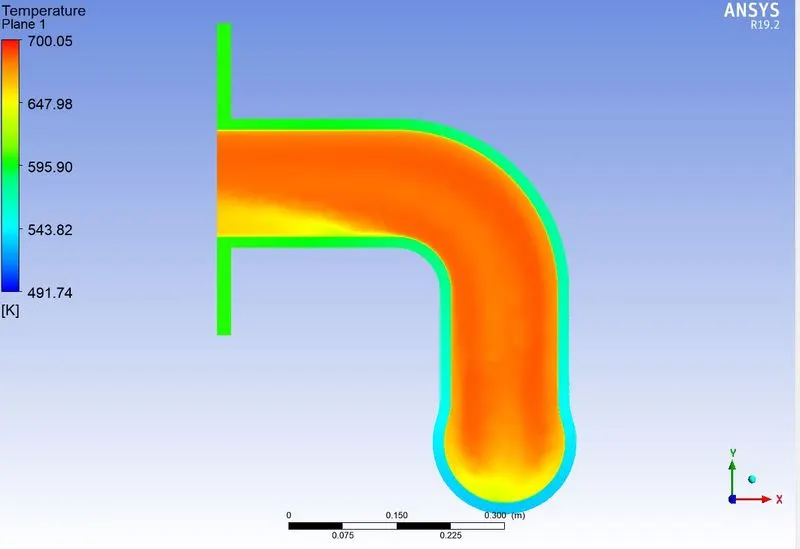
• Then go to the results to get appropriate plots such as velocity contour and temperature contour.

Outputs:

First Refinement:

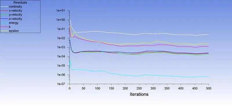
Residual:

Velocity Contour:

Temperature Contour:

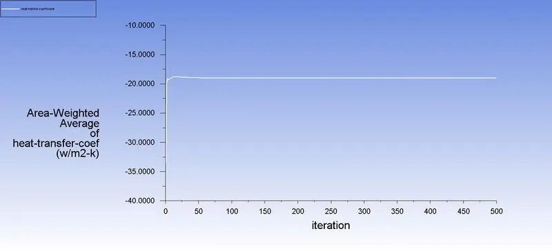
Heat Transfer Coefficient plot:

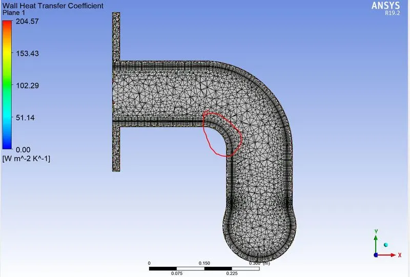
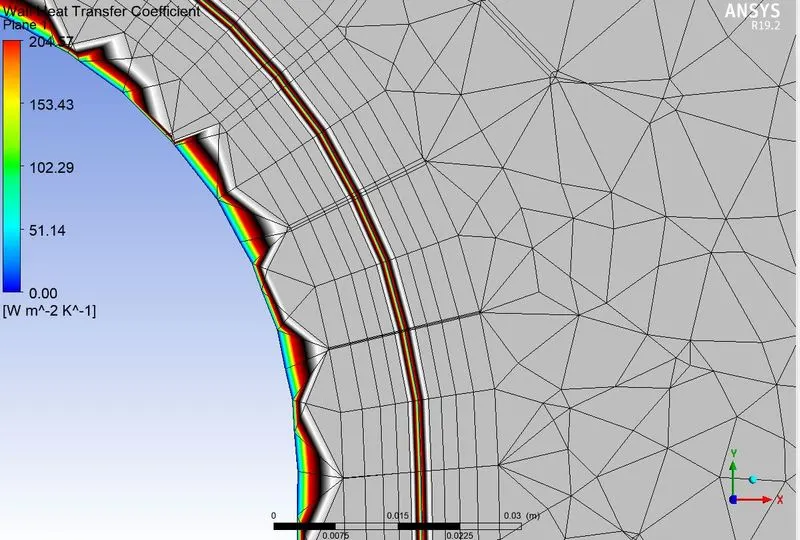
Heat Transfer Coefficient:

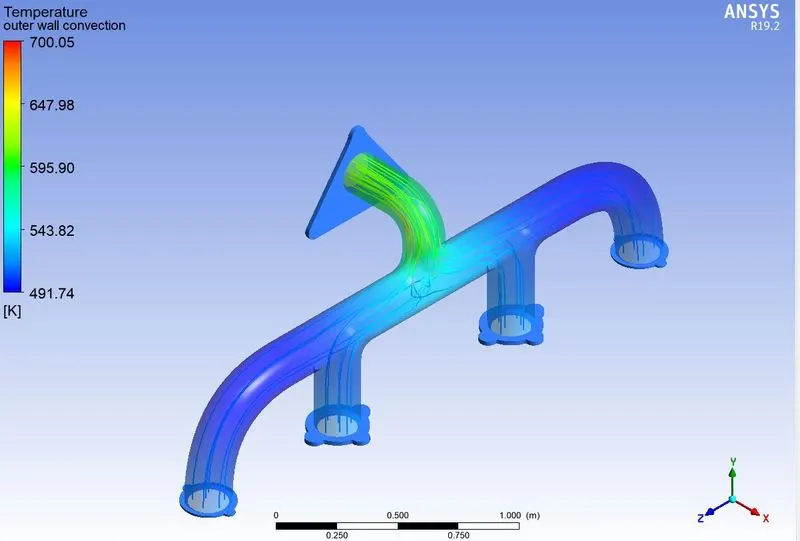
Temperature Streamline:

Second Refinement:

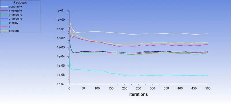
Residual:

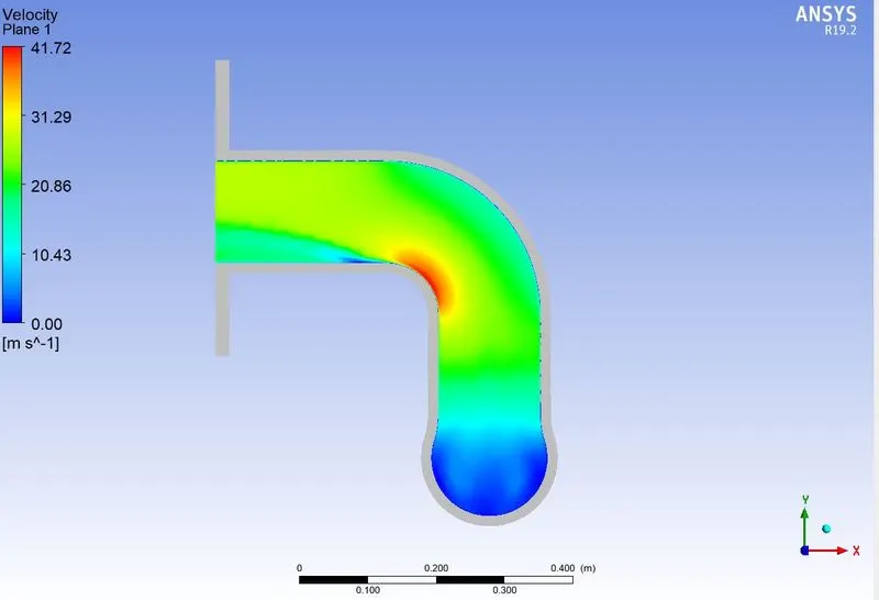
Velocity Contour:

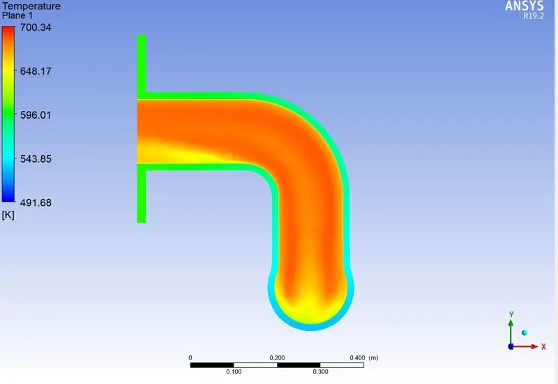
Temperature Contour:

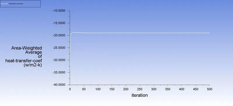
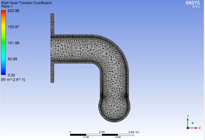
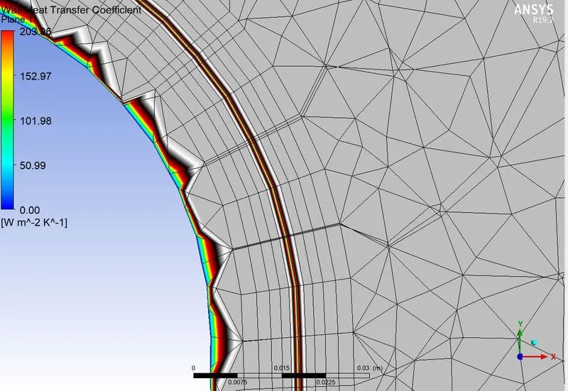
Heat Transfer Coefficient plot:

Heat Transfer Coefficient:

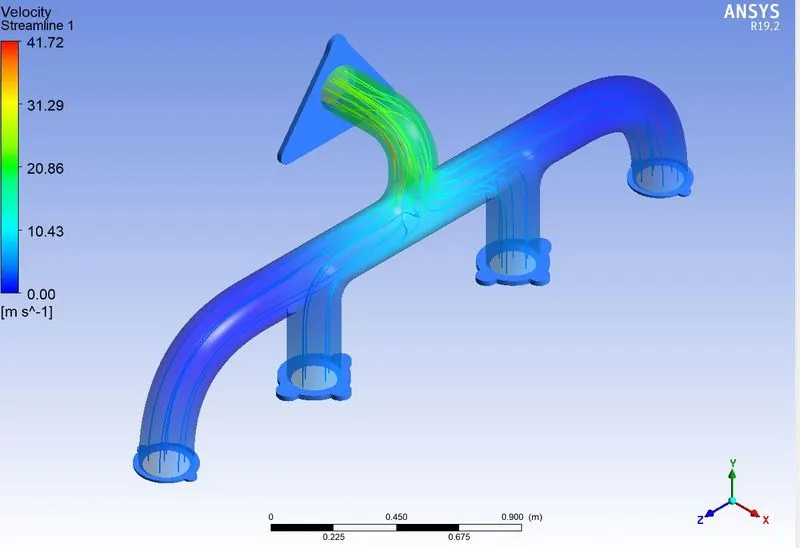
Velocity Streamline:

Third Refinement:

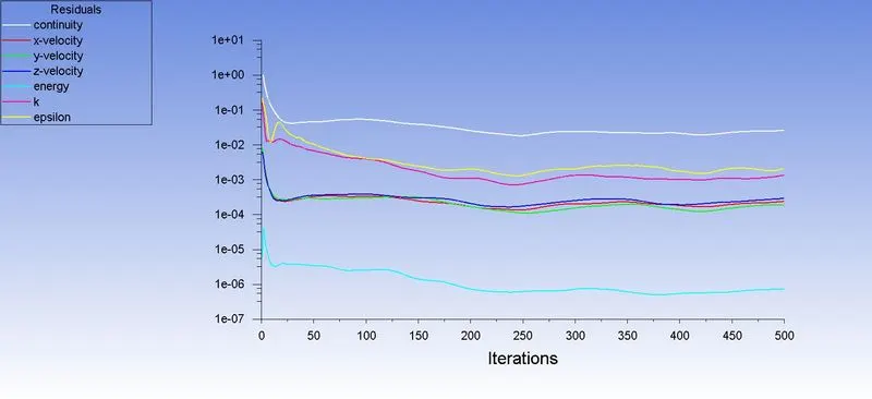
Residual:

Velocity Contour:

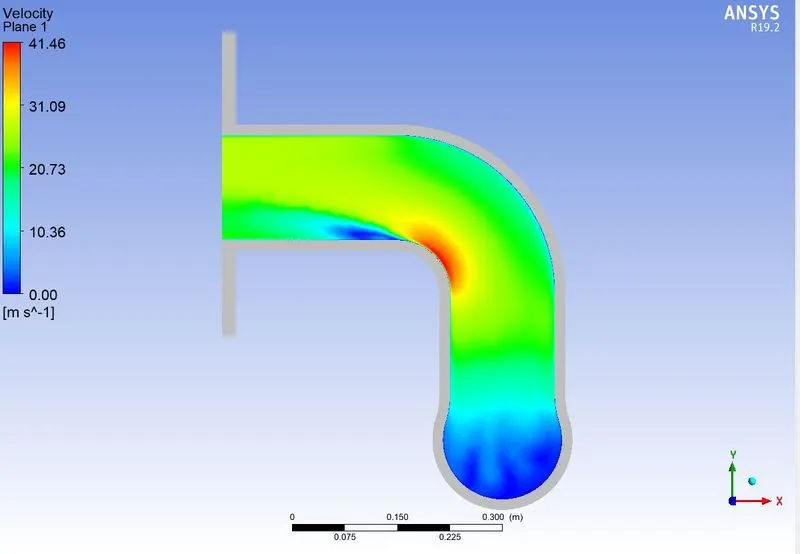
Temperature Contour:

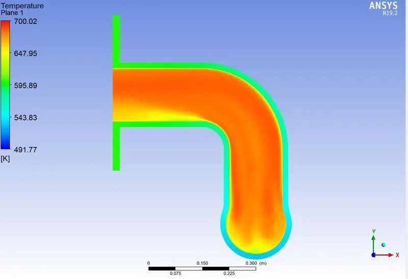
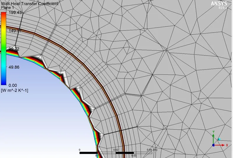
Heat Transfer Coefficient plot:

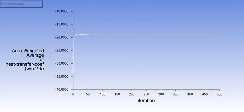
Heat Transfer Coefficient:

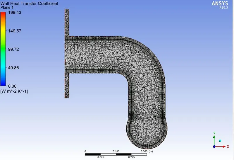
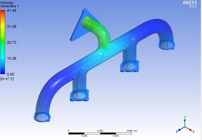
Velocity Streamline:

Refinement	Mesh Size	Nodes	Element	Heat Transfer Coefficient
1st refiement	90	397338	1120063	19.8
2nd refinement	80	396866	1118854	19.9
3rd refinment	70	397189	119764	19.8

Verify HTC :

• Under forced convection circumstances, we can determine the heat transfer coefficient by using the Dittus-Boelter
  correlation. Using the Dittus-Boelter correlation the heat transfer coefficient can be calculated in the following way using
  two further dimensionless groups, the Reynolds number and the Prandtl number.

`h = (k/D )*Nu`

• where k is the thermal conductivity of the liquid, D is the Hydraulic diameter, and Nu is the Nusselt Number which is
  determined by the following equation,

`Nu = 0.023Re Pr`

• where, n= 0.4 when fluid is being heated
  n= 0.3 when fluid is being cooled

In this equation, Re is the Reynolds number which equates to,

`Re = (m D )/(μ)`

• and Pr is the Prandtl number,

`Pr = (CP* μ)/k`

• For the Reynolds number, m is equal to the mass flow rate. For the Prandtl number, C_Pis equal to heat capacity, and in both
  equations, μ is the viscosity of the fluid in consideration. Once we have all of these factors, we can get a decent
  estimation of the heat transfer.

Accuracy of HTC prediction :

Accuracy of the predictions depends on several things like,

1. Accurate geometry of model.

2. Its Mesh quality.

3. Inflation layers

4. Properties of material being used.

5. Turbulence models.