Week 4 - CHT Analysis on Exhaust port

THE AIM: To analyze conjugate heat transfer through on exhaust manifold.

INTRODUCTION: conjugate heat transfer analysis is based on mathematically structured problem, which describes the heat transfer between a body and a fluid flowing over or inside it as an interaction between two objects.

Conjugate heat transfers correspond with the combination of heat transfer in solids and heat transfer in fluids. In solids, conduction often dominates whereas in fluids, convection usually dominates. Efficiently combining heat transfer in fluids and solids is the key to designing effective coolers, heat exchangers. Forced convection is the most common way to achieve high rate.

THEORY: though conjugate heat transfer help us to analyze heat transfer between solids and fluid, it has some of the formulas from where we can find out the answers numerically and compare it with our analytical results. Here in our experiment, we have the problem from convection so the formulas for numerical validation are used below

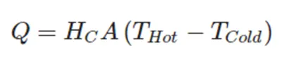
Where Q is heat transferred Hc is heat transfer coefficient

A is the area

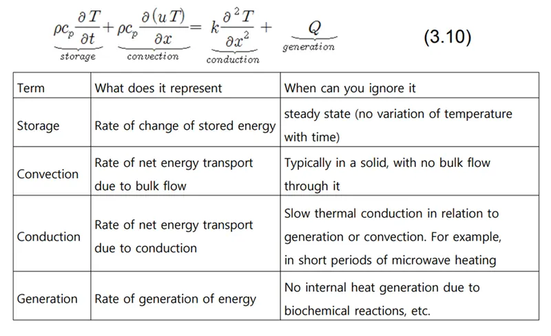
This is governing equation for heat transfer derived from energy conversation and Fourier law. though we are not going to use this complex equation we have a direct relation of Nusselt no. with Reynolds no. which we will discuss further.

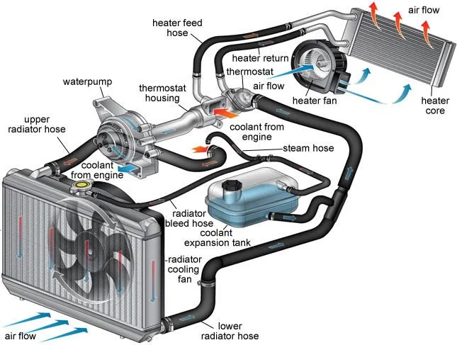
Application: the conjugate heat transfer methods have become a more powerful tool for modeling and investigating nature phenomenon and engineering systems in different areas ranging from aerospace and nuclear to our household and also over a vast medical faculty. basically, used in the engines of car bikes etc., also in the manufacturing of pipes, wires etc., in recent years the improvement of the cht in cooling performance of electronics such as the design of refrigerators, air-conditioners, and various heat exchangers for waste treatment plant is significant.

SOLVING AND MODELLING APPROACH:

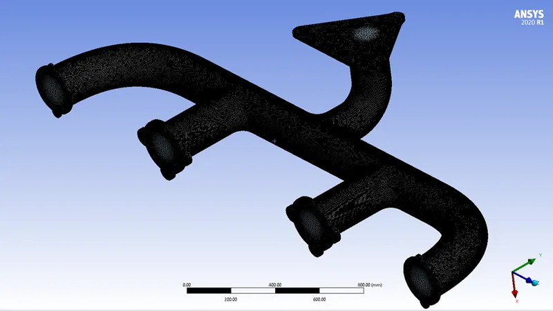
So, we divided this case in two approaches that is the coarse mesh and the refined mesh, so we have to open the spaceclaim and then have to repair our geometry because there are some extra edges. After that we have to specify the solid and fluid volume and change our geometry topology into share this will make our mesh quite more good help us to capture better results. The geometry and solving settings that we are going to use are shown below:

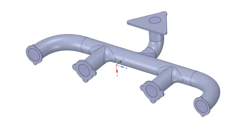
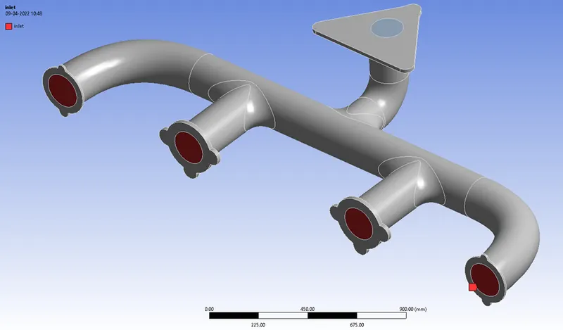
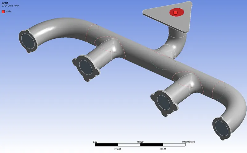
So, this our geometry the diameter of every hole (inlet and outlet) is 0.1661m which will be our characteristic length for this case to solve the Reynolds no.

Inlet,

Outlet,

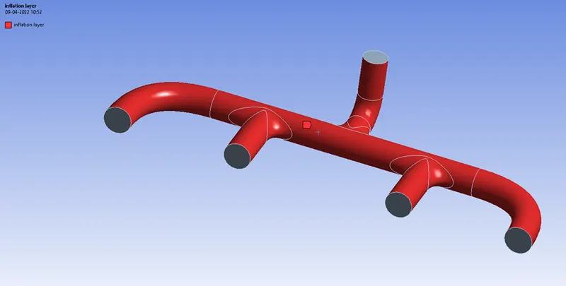
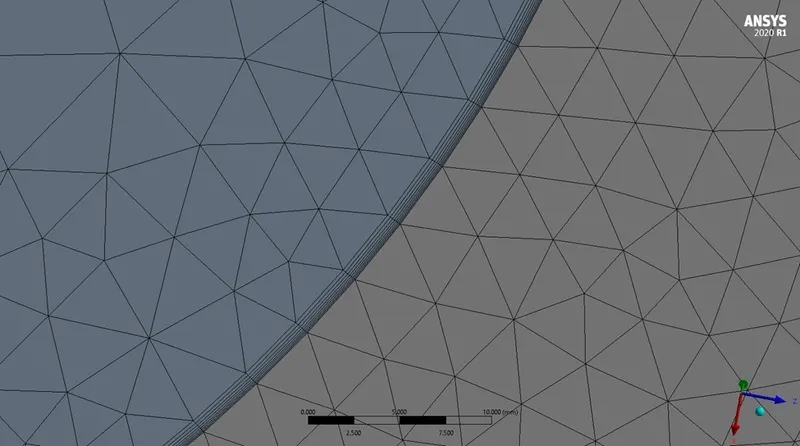
Inflation that we will use for the refined case,

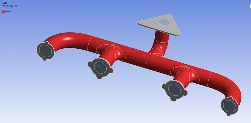
And the walls,

After that lets discuss about the modal we are going to use and why?

So, the turbulence modal that we are going to use is k omega SST modal because it is designed to be applied throughout the boundary layer. It also uses the near wall approach rather then wall function approach (used by k epsilon standard turbulence modal).

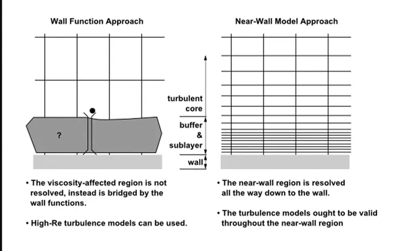
So, after that we have to use the y-plus value, basically it depends on the k-omega and k-epsilon modal as per the law of the wall. The y-plus value for k-omega modal should be between 0-5 while as for k-omega modal it should be in between 30-300 range.

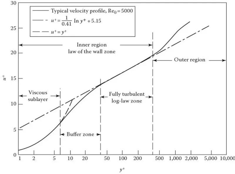
The graphs are based on log-log plot so the straight line is logarithmic while the curve line is linear.

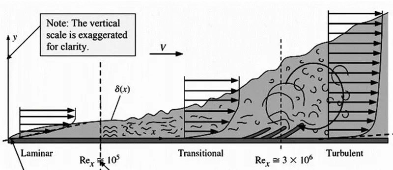
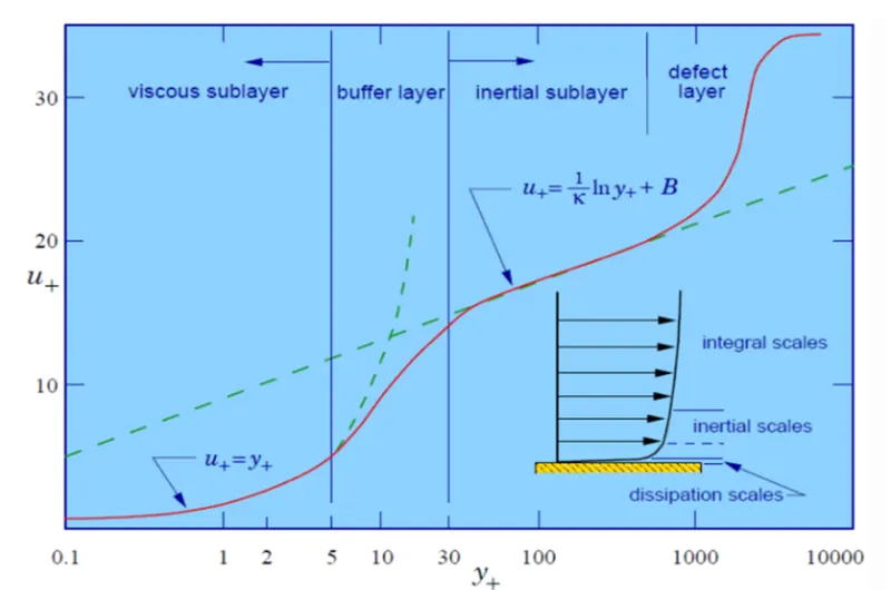
So, I use two graph to specify this that our modal will in range of 0-5 that is viscous sublayer.

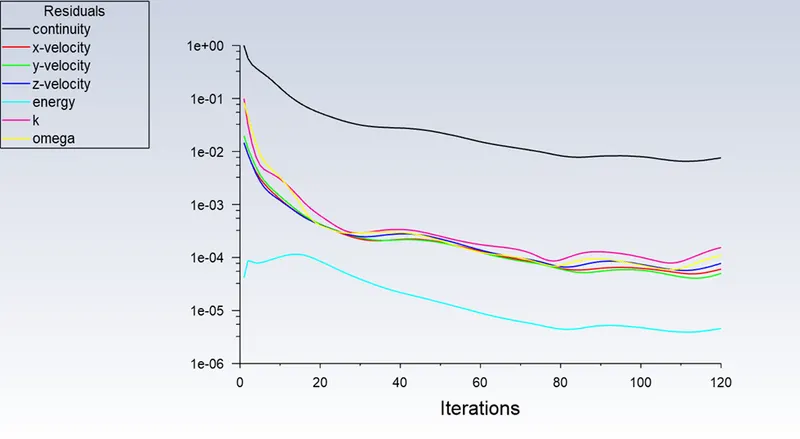
The no. of iterations will be different because when we run the coarse mesh the plots show us where will be the convergence according to that we can reduce and increase the no. of iterations although it depends case by case the time step for each iteration will be 1.

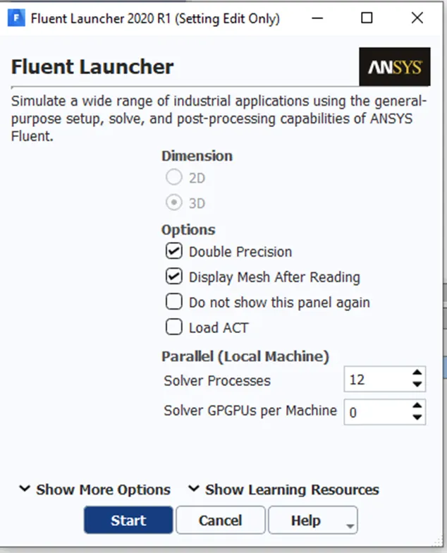
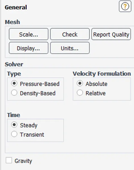
We are going to use the general setting as pressure-based solver, velocity formulation should be absolute and time should be steady

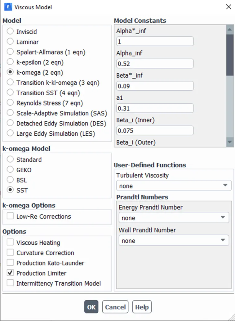
PRE-PROCESSING AND SOLVER SETTING:

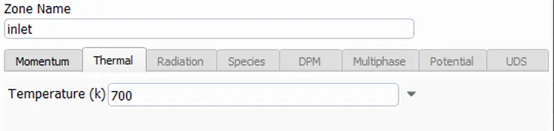
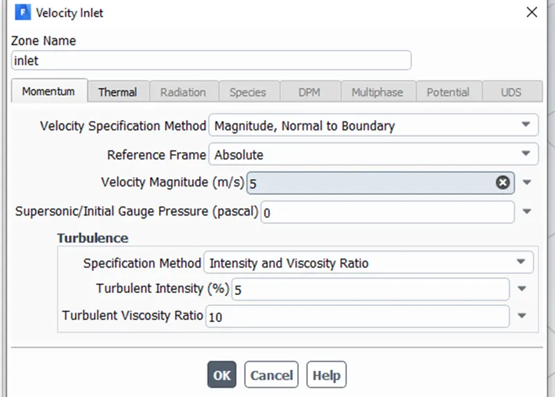
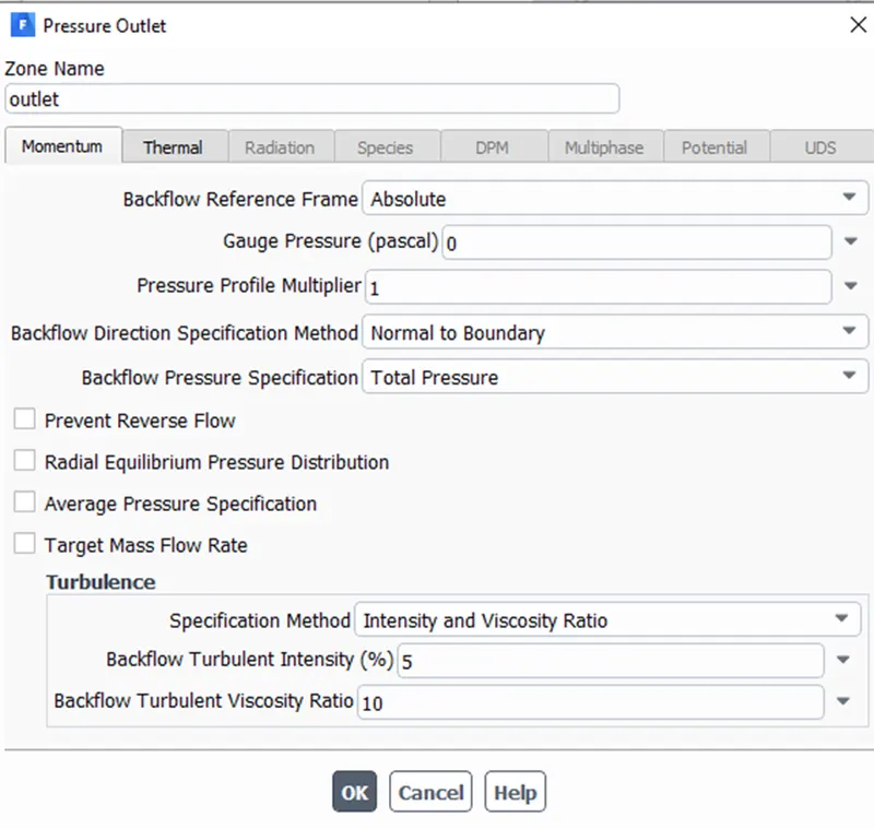
1^st of all let’s talk about the boundary conditions, at inlet the velocity is 5 m/s and the temperature is 700k. on the other hand at outlet the gauge pressure is 0.

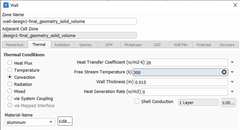
The heat transfer coefficient is 20 w/m^2-k is 20 at free stream temperature 300k and the thickness of 0.015m.

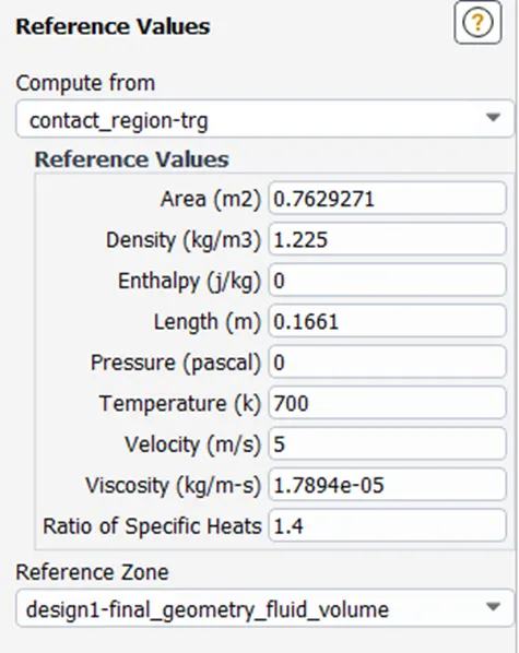
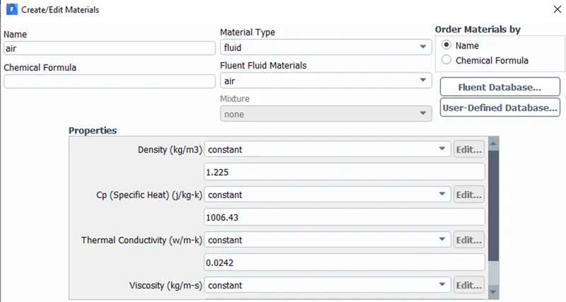
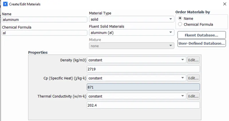
Material properties are given below we use two material one of them is air as our fluid whereas for the wall the material is aluminium.

After the basic settings and the properties of material we are going to shift ourself toward our cases

Case1:

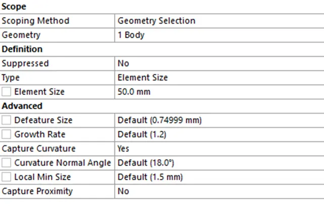
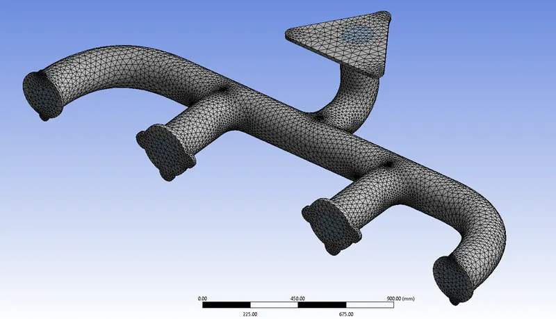
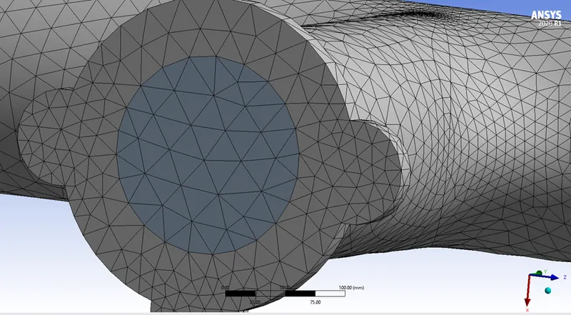
In this case we have very basic mesh and no inflation layer the element size is 50mm for the mesh. The no. of nodes is 33400 and no. of elements are 136967.

The element metric is given below,

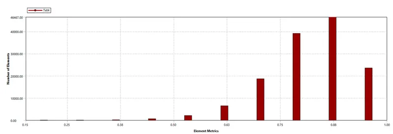
So, from the images we can see the mesh is quite coarse.

Case 2:

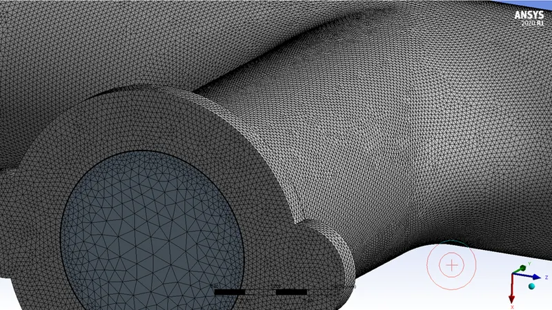
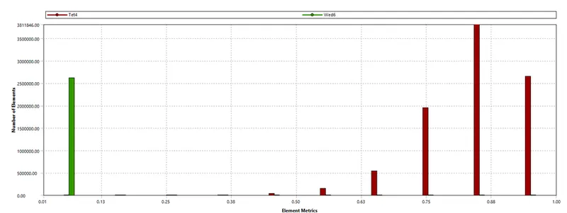
In this case we have inflation layer and have refined mesh and the element size of 20mm whereas the sizing of the whole geometry is 4mm, and then for the inflation layer the size of the first layer is 0.0514392mm and have growth rate of 1.2 with 8 inflation layers the total thickness 0.8486997228mm for the complete mesh. The no. of nodes is 3116602 and the no. of elements is 11753668. And these are the value which is useful to maintain the y plus value of 1.

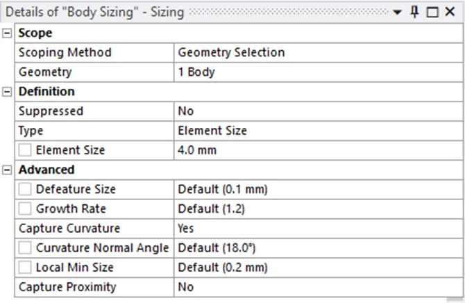
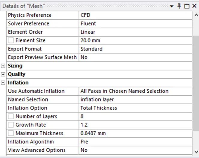
The element metric is given below,

These are the properties and the mesh settings that we are going to use to solve our problem.

Cases	No. of nodes	No. of elements
Case 1	33400	136967
Case 2	3116602	11753668

RESULTS: here we are going to discuss about the contours and plots which will help us to find the analytical value of our cases;

CASE 1: in this case we have a mesh of element size of 50mm. this case will give us the idea how we have to maintain the y+ value along with better mesh and show us that how much iterations are required for convergence although it gives us a huge deviation in answer. The plots and the contours are given below:

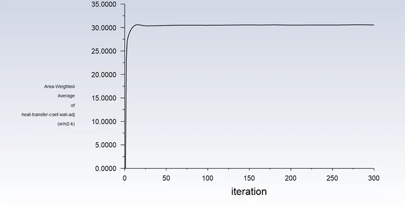
Area weighted of heat transfer coefficient wall adjuctive: 30.498422 w/m^2-k

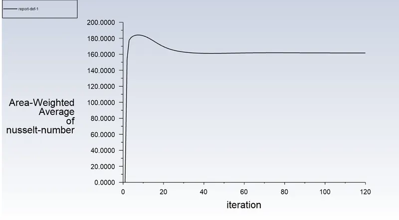
Nusselt no.: 161.64462

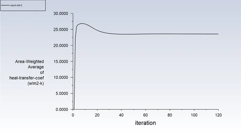
Area weighted average of heat transfer coefficient: 23.550872w/m^2-k

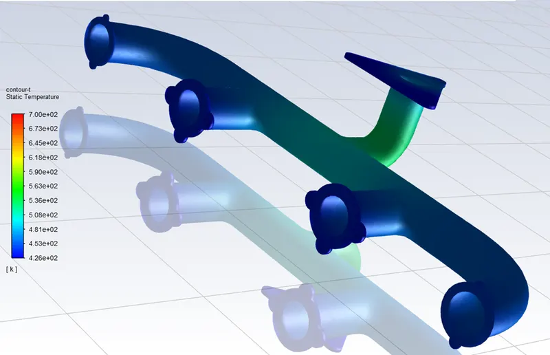
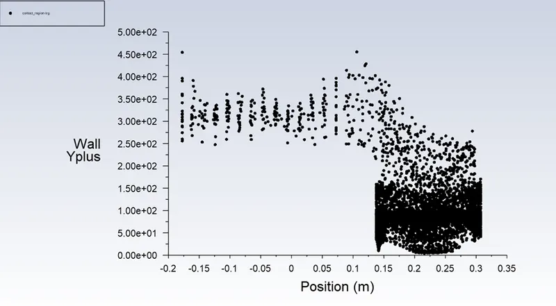
Here we can see that y+ value in this case not maintained and also here is a lot more deviation in area weighted average of heat transfer coefficient wall adjective. The value is 30.498422w/m^2-k.

Whereas the experimental value for this is around 980 w/m^2-k. and the velocity at the outlet is 25.237047m/s so we can see that the velocity at the inlet (5m/s) and at outlet is completely different.

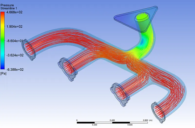
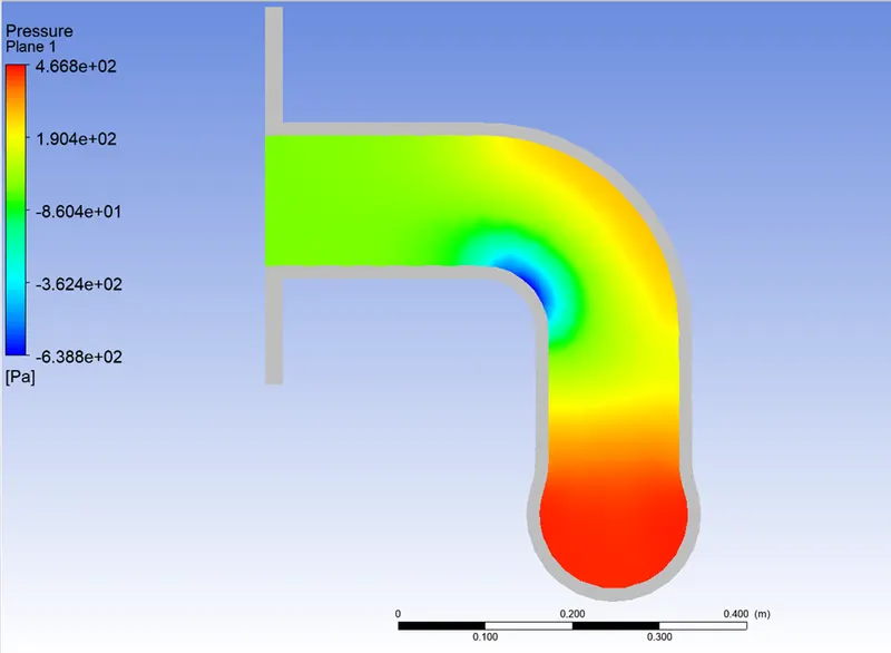
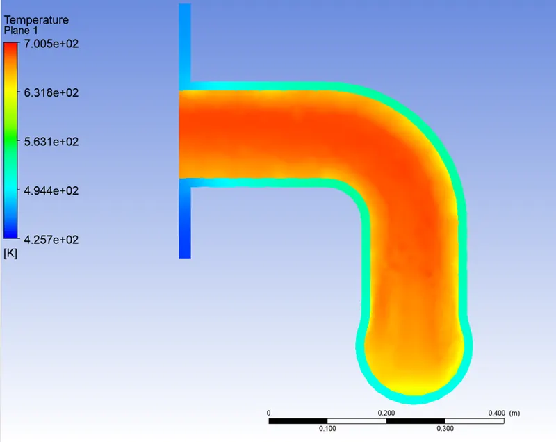
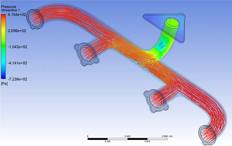
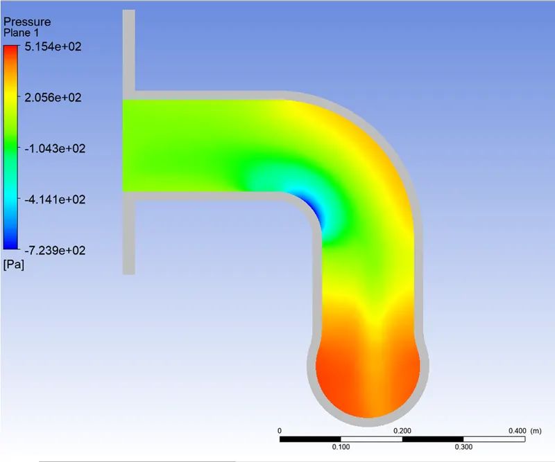
The streamline for velocity, pressure and the temperature are given below along with the contours of wall heat transfer coefficient, wall heat flux.

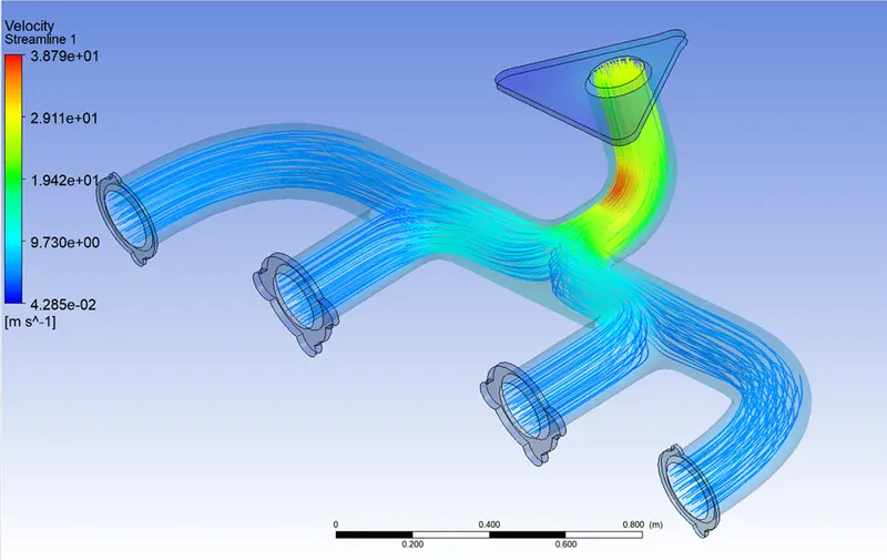
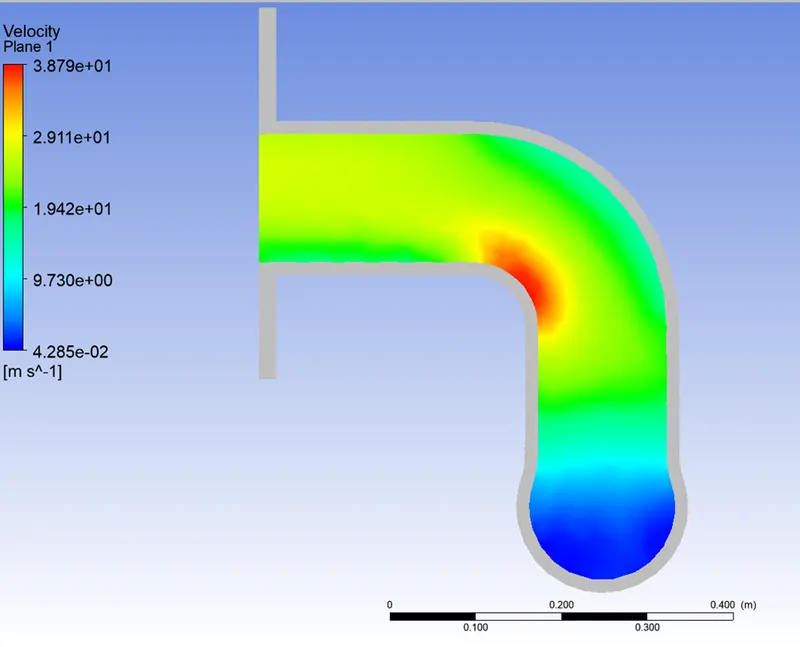
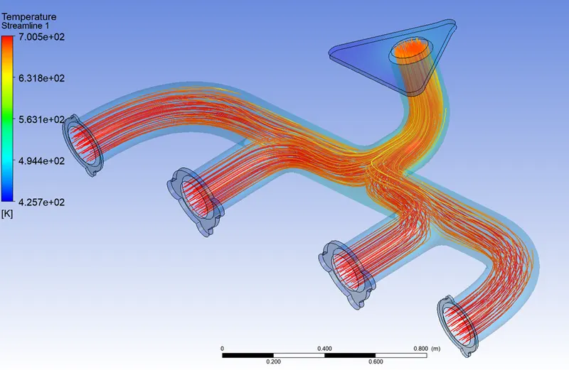
The temperature at the outlet :678.2619K

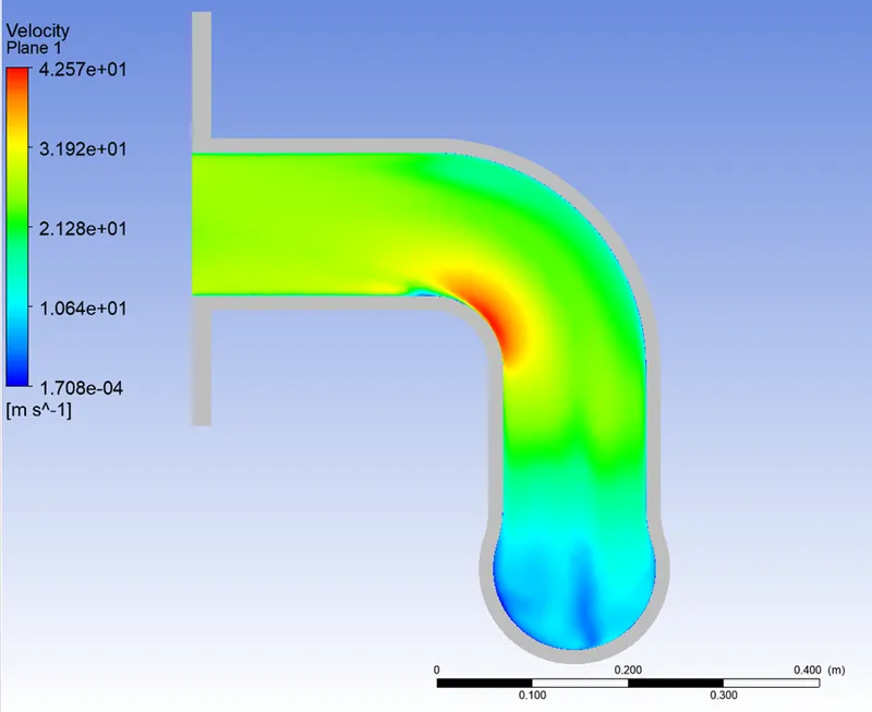
The vector contour for the velocity is given below,

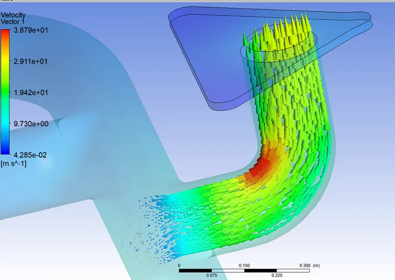
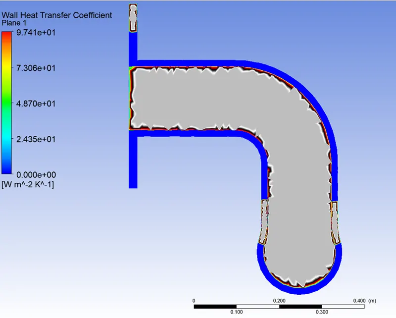
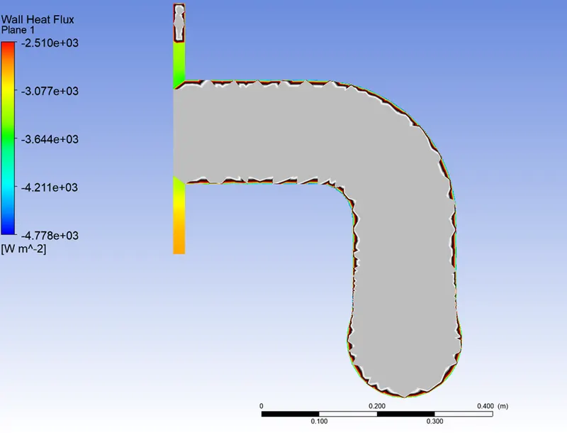
From the contours we can see that velocity is high at the turning point, the temperature at this point is also very high. Hence the area weighted average of heat transfer coefficient is 23.550872w/m^2-k whereas the numerical answer is 18.9537457981w/m^2-k having approx. 24.2544468564% error.

Heat transfer Q: 6782.3482424339 watt (31.595411991%error)

CASE 2: in this we have a refined mesh having body sizing of 4mm and inflation layer of total thickness of 0.8486997228mm with 1.2 rate of growth. For this we maintain the value of Y+ to be 1 that is in between 0-5 which is very good for k-omega SST turbulence modal. The plots and contours are given below in this case the refinement is very high so the answer will be near to our experimental value,

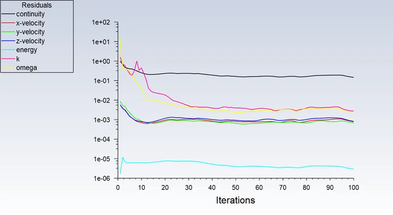
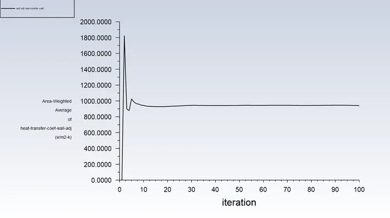
The area weighted average of heat transfer coefficient wall adj.: 942.0365w/m^2-k.

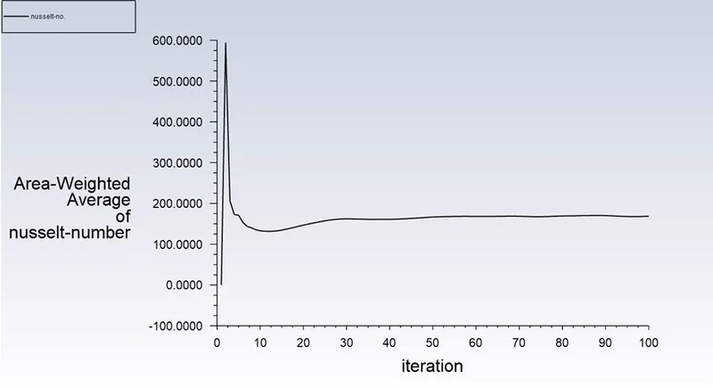
Nusselt no. :168.57725.

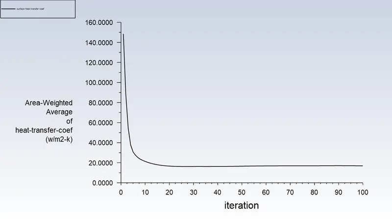
Area weighted average of heat transfer coefficient:

16.971332w/m^2-k.

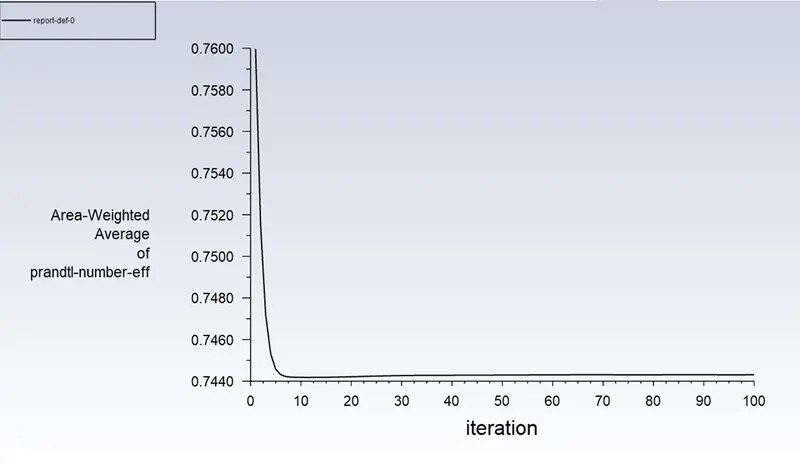
Prandtl no.: 0.74430948

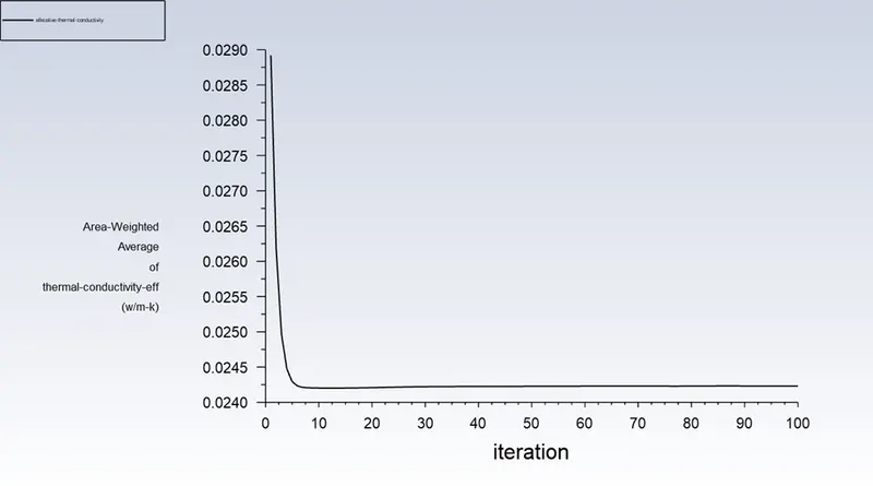
Thermal conductivity effect is analysed as the result is 0.024231618w/m-k

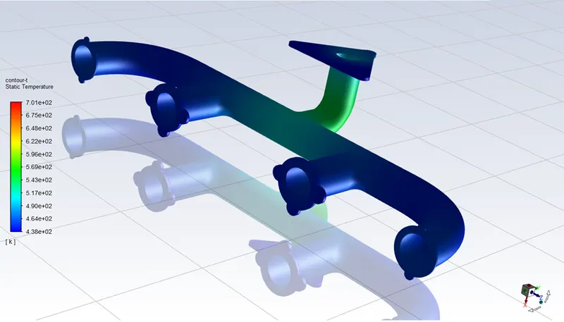
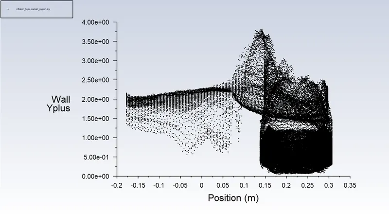
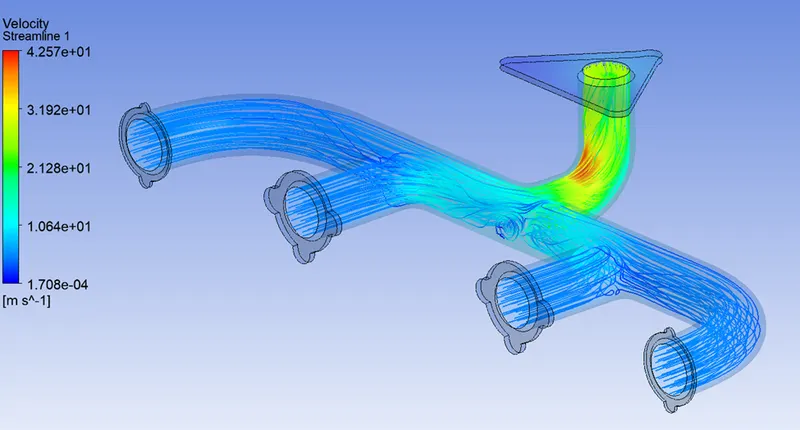
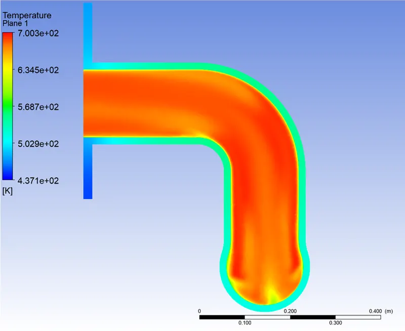
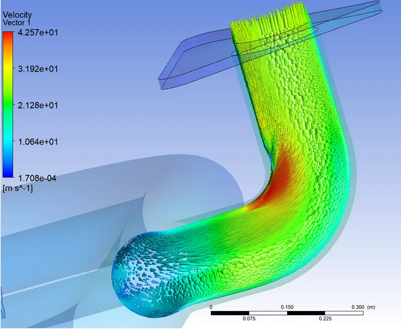
Here in this case, we can clearly see that the Y+ value is maintained and is between the 0-5 range it is because we choose the right thickness of inflation layer. And we can see that there is a very less percentage error in between the experimental value and the analytical value of area weighted average of heat transfer coefficient wall adj. the value of the analytical result is 942.0365w/m^2-k and having a deviation of 3.878265306% error. The velocity is 25.157012m/s at outlet. So, we can see that the velocity at inlet is totally different this because the velocity at the inlet is mixing up and the result will give us high amount of change and from the streamline view, we can see that at the turn where the fluid will mix and approach to the outlet, we can see that where the velocity is maximum the temperature or the heat transfer at that point is also more then average. The contour and the stream line along with the contours of wall heat transfer coefficient, wall heat flux is given below:

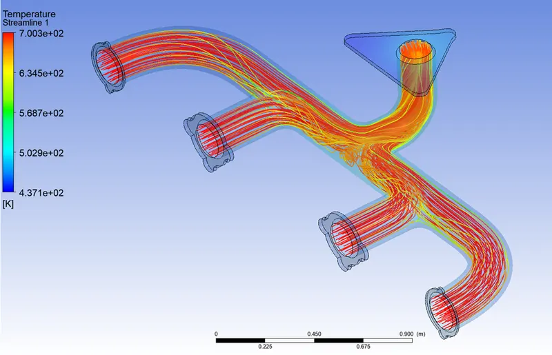
The temperature at outlet is 682.001 k.

The vector contour for the velocity is given below,

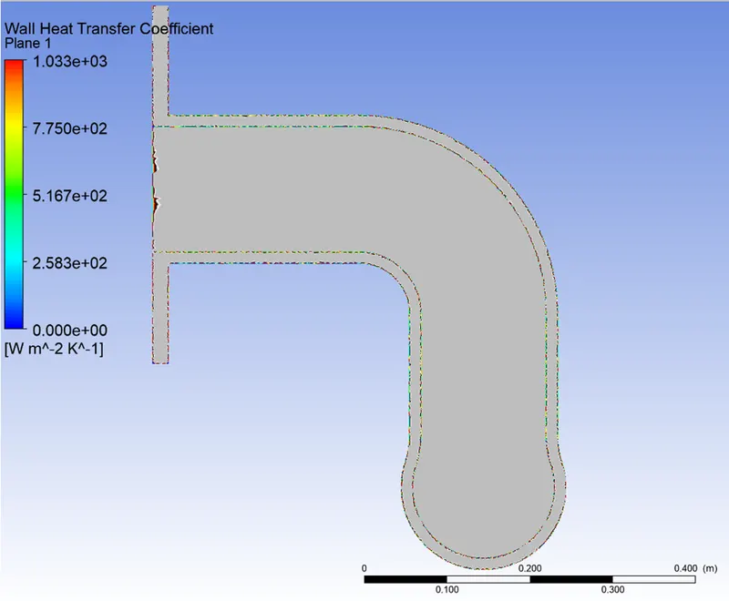
Wall heat transfer coefficient,

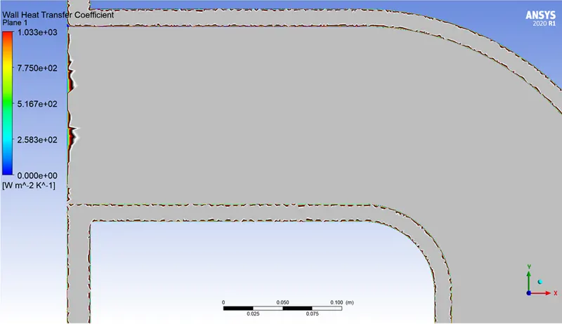
Wall heat flux,

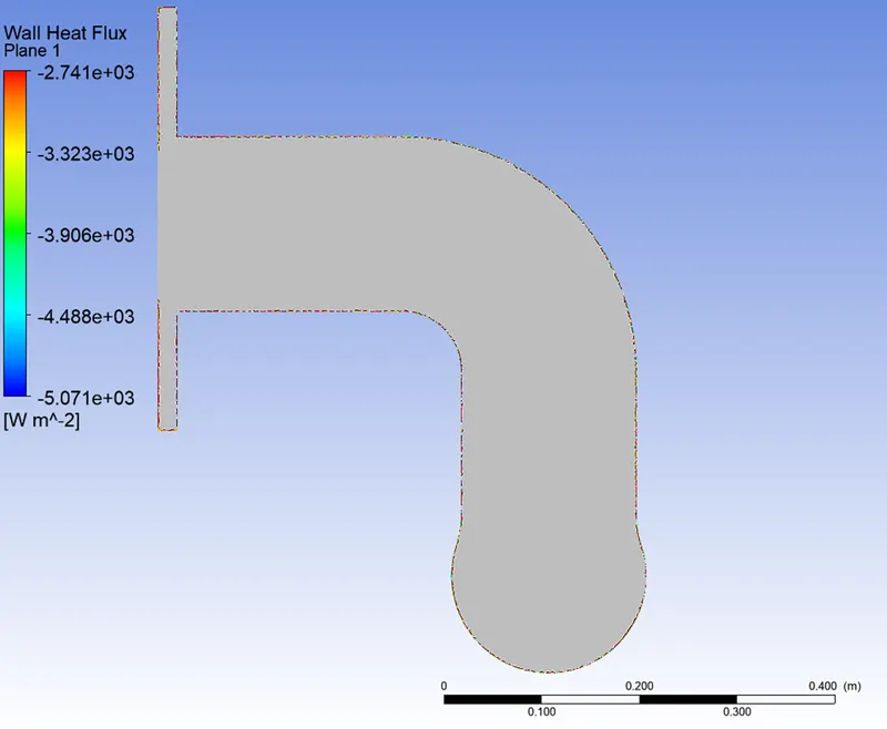
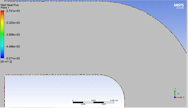
Hence the area weighted average of heat transfer coefficient is 16.971332w/m^2-k whereas the numerical answer is 18.9537457981w/m^2-k having approx. 10.4592190864% error.

The area weighted average of heat transfer coefficient wall adj.: 942.0365w/m^2-k (3.8738265306%error)

Nusselt no. :168.57725 (29.5834823507%error)

Area weighted average of heat transfer coefficient:

16.971332w/m^2-k. (10.4592190864%)

Thermal conductivity effect is analysed as the result is 0.024231618w/m-k (0.1306528926%error)

Prandtl no.: 0.74430948 (0.045967742%error)

Heat transfer Q: 4935.8387067352(4.2317343507%)

NUMERICAL VALIDATION:

We just conclude our analysis here and to verify this all we have to calculate the thermal and heat transfer coefficient. We have to calculate from the formula of Nusselt no. Nu=hl/k where is the heat transfer and we can also calculate the heat transfer by the formula

So, we have to find the h we have to find the Nusselt no. after that from Dittus-Boelter equation

Nu=0.023*(Reynolds no.^ (4/5)) *(pr^n).

Where Nu is Nusselt no., Prandtl no.’s n is 0.4 when the fluid is heated and 0.3 when the fluid is cooled off.

So, for numerical answers we are going to use some values and some given formula

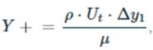
Cf=0.0576*(Re^ (-1/5))

So, from all this we will get the inflation layer and give a proper thickness of inflation layer and maintain the Y+ value for our case. Reynolds no is 56867.663499161

For the properties of air

K is the thermal conductivity of the material is 0.0242w/m-k

Pr =0.744

N is constant 0.4 heat transfer takes place from fluid to solid (0.4 because fluid is heated).

Convection heat transfer coefficient h = Nu*k/Lc

Nu no. for these cases is 130.0916188869

And h for these cases is 18.9537457981w/m^2-k.

And the Q the heat transfer is 5153.9397435356 watt,

The experimental result of the heat transfer coefficient wall adj 980 w/m^2-k.

So, we are going to compare the analytical values here and choose where our analysis is right or not.

	Numerical value or experimental value	Case 1	Case 1 error percentage	Case 2	Case 2 error percentage
heat transfer coefficient wall adj	980 w/m^2-k	30.498422 w/m^2-k	96.8879161224%	942.0365w/m^2-k	3.8738265306%
heat transfer coefficient h	18.9537457981 w/m^2-k	23.550872w/m^2-k	24.2544468564%	16.971332w/m^2-k	10.4592190864%
Heat transfer Q	5153.9397435356 watt	6782.3482424339 watt	31.595411991%	4935.8387067352 watt	4.2317343507%

COCLUSION:

• We can see the huge deviation in the coarse mesh where we don’t have inflation layer
• Inflation is required to capture the near wall phenomena
• We concluded that the perfect knowledge of the mesh solver is required for the CHT analysis
• The finer mesh has quite better results than the coarse mesh we can see the deviation range of refined mesh is between 0 to 10% for all the three cases discuss in the table
• Our analysis of CHT is quite successful because of the less deviation
• Y+ should be maintained according to the solver, for k-omega SST turbulence modal it should be between 0-5 whereas for k omega standard modal it is between 30 to 300.
• Also, we have to choose the modal according to our approach in these cases the we have to choose the near wall approach rather then the wall function approach
• The velocity at the outlet is higher the velocity at the inlet and we can see it clearly in the contours.
• The large deviation in the analytical result and numerical is because we neglect some values while do the numerical validation or vice versa.
• The presence of boundary is visible as we can see at the inlet where the viscous force near the wall make the velocity 0 we can observe that the no slip condition is quite effective there, but the flow is turbulent the velocity profile becomes flutter after some time and completely vanished at the outlet.
• The result are quite good because we don’t neglect the small things like the accuracy of the area, providing thickness which resulted in quite better results.