Week 3 - External flow simulation over an Ahmed body.
THE AIM: So, in this we are here to discuss the flow over an Ahmed body and try to explain the negative pressure in the wake region, also the significance of the point of separation. For all the cases we will maintain the Y+ between 30 and 300, so basically, we divide the cases for different y+ value to get the required result of drag coefficient (0.33) and from the reference papers try to calculate the result of drag as well (0.283).
INTRODUCTION: The Ahmed body is a generic car body (a simplified vehicle model). The airflow around the Ahmed body captures the essential flow features around an automobile and was first defined and characterized in the experiment work of Ahmed. Although, it has a very simple shape, Ahmed body allows us to capture characteristics feature that are relevant to bodies in the automobile industry. This model is also used to describe the turbulent flow field around a car like geometry. Once the numerical model is validated, it is used to design new model of the car.
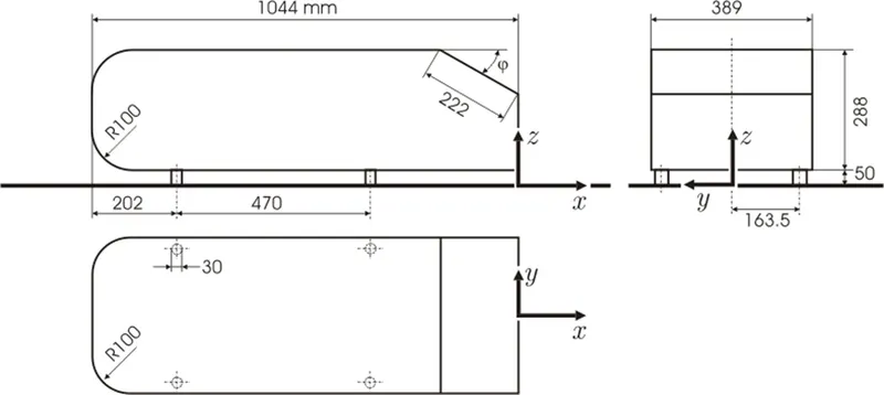
The length of this model should be 1044 mm but when I calculated and simply measure the length was around 1048.78mm so for this project we use this length and the projected area of the body according to this length is 0.131482mm.
THEORY: the Ahmed body was created by S.R. Ahmed in his research “some salient features of the averaged ground vehicle wake” in 1984, Since then it has become the benchmark for aerodynamic simulation tools. It has simple geometry including length of 1.044 m and height of 0.288 m and width of 0.389m. this body is enough to model, while maintaining car like geometry features.
Airflow over the body: so, we have a body with a calculated length of 1.04878m and projected area of 0.131482m. the Ahmed body has slant of 25, whole the calculation will be done in a domain of 8.39024m*1.389m*1.04878m
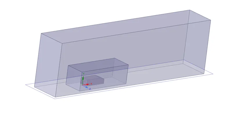
So, from the diagram we can see there is two domains the volume of the bigger domain is 8.39024m*1.389m*1.04878m and the volume of smaller domain is 2.62195m*0.911m*0.52439m. so these are our domain in which the bigger domain will have a course mesh then the smaller one so that we will able to see every effect of simulation. Simply the air will flow from the inlet with 25m/s of velocity and we will use all the default settings.
The flow of this model is basically turbulent, the simulation solves the turbulent kinetic energy and dissipation in addition to the velocity and pressure field.
So, from the drag force we will able to know that all are cases work well, and that will made up of measurements for the pressure coefficients in the front, slant and base as well as the body’s skin friction. From our simulation we will get the result with minimum error percentage but the individual measurements deviate from the experimental result is varying amounts, like there will be some deviations like we are not able to predict the flow transition for the front and the roof, in our experiment we try to see the recirculation zones which will we created behind the body. But we will not be able to predict the zone that how much will we its extent
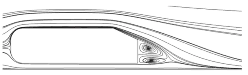
So, this will be the zone that we will see in the cases. Hence the pressure drag for the slant coefficient is very sensitive to exact shape of the recirculation region, which will show some error although it gives us the less error drag coefficient.
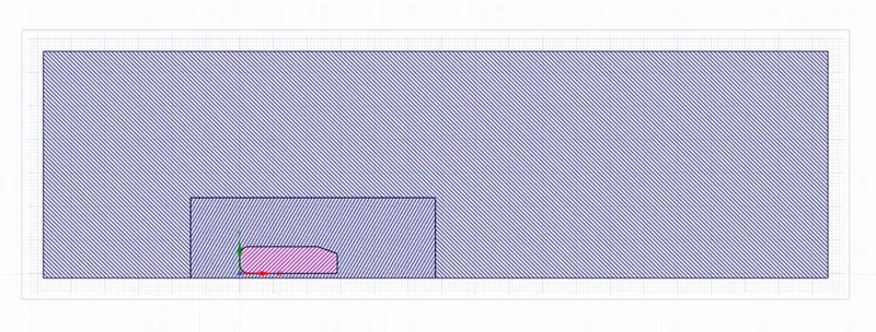
SOLVING AND MODEL APPROACH: so first we import our geometry in the space claim, and after that make encloser of volume 8.39024m*1.389m*1.04878m. after that we create and another encloser within this domain encloser of volume2.62195m*0.911m*0.52439m. so after that we just check that is there any overlapping in our geometry for that we use interference tool and remove every overlap line after that we check the topology which should we in share so that there will no difference in both the enclosers. Should look like given image:
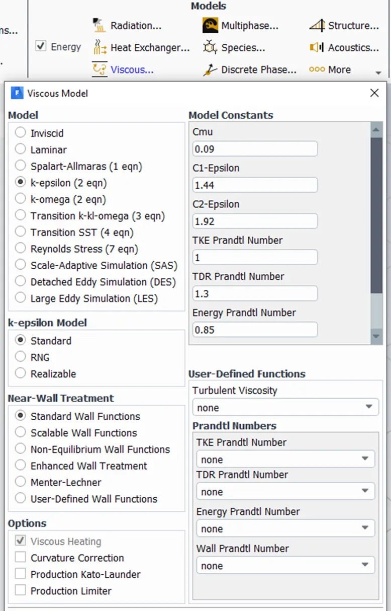
After that we go for meshing, so from here we prepare different cases for different Y+ values so 1st the case should be run in total default settings after that our second case setting should be differ according to 6 different Y+ values, also give named selection according to inlet face outlet face, car wall and symmetry wall. And also, for method for large encloser we choose the multizone method and values can be differ case by case as shown in given table, after that we give the sizing for the inner/ small encloser which can also be differ case by case and for that support we choose a constant value in sizing for all the cases 3mm except the last case which will be 2mm and growth of layer must be 1.1 for each and every case. After that we will run our fluent in which we use the k epsilon modal of viscous.
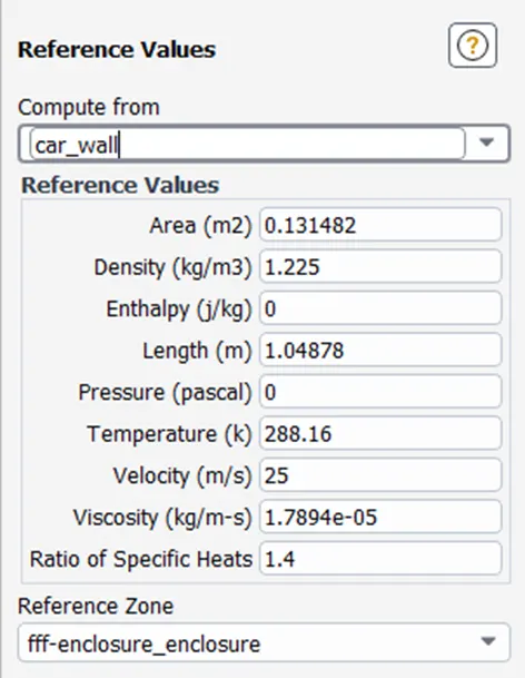
give all the reference values that are required to solve the problem
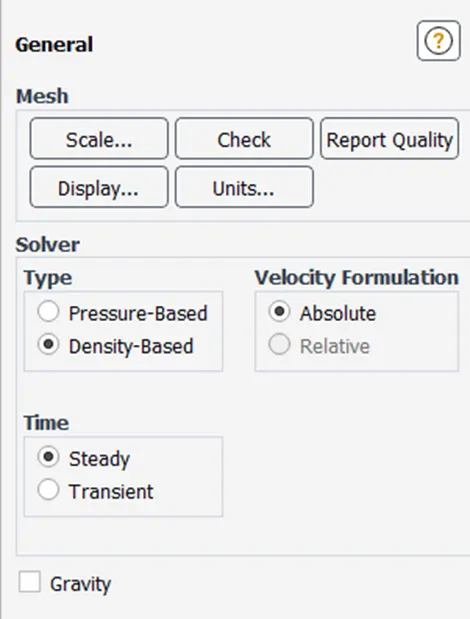
, the solver should be steady and density based.
After that, we also use the hybrid model for initializing we prepare a plane and from that plane we prepare the contours.
So, from this all our preparations to solve the cases are ready. Now for all the cases we have,
|
No. of cases |
Y+ value |
First layer thickness mm |
No. of layer |
Total layer thickness mm |
|
1 |
nil |
1 |
6 |
7.71561 |
|
2 |
70 |
1.0034039 |
7 |
9.519464343814 |
|
3 |
110 |
1.5767775 |
8 |
18.0318510486 |
|
4 |
160 |
2.2934946 |
9 |
31.1444569639 |
|
5 |
220 |
3.153555 |
10 |
50.2595450376 |
|
6 |
270 |
3.8702721 |
11 |
71.720658857 |
|
7 |
290 |
4.1569589 |
7 |
39.4377749243 |
|
No. of cases |
No. of nodes |
No. of elements |
Element size of outer encloser mm |
Element size of inner encloser mm |
Element size of cylindrical body support |
|
1 |
50579 |
161309 |
440 |
440 |
3 |
|
2 |
66548 |
173923 |
120 |
60 |
3 |
|
3 |
99144 |
259428 |
100 |
50 |
3 |
|
4 |
151124 |
399968 |
80 |
40 |
3 |
|
5 |
202057 |
547132 |
70 |
35 |
3 |
|
6 |
372307 |
1207315 |
60 |
25 |
3 |
|
7 |
969087 |
4596187 |
60 |
15 |
2 |
So, from this we have now an idea of how we will goanna solve all our problems. Then after we just have to open the result and see the vectors and also prepare charts of u velocity-y chart, although we will see every result of all the cases in the results section. And I have to specify that the case 1 is not a refined case so we also don’t choose any Y+ value to give the first layer thickness.
PRE-PROCESSING AND SOLVER SETTING:
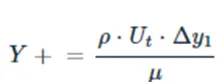
So, we got all the things ready now we have to calculate the Reynolds no., Ut skin frictional velocity, shear stress and skin friction factor from this above value we got the delta y1(first layer thickness for each case w.r.t Y+).
So, for calculating these we have characteristic length of 1.04878m, velocity of 25 m/s, density of 1.225 kg/m^3 and dynamic viscosity of 1.7894e-05 kg/m-s. and the formulas are given below as:
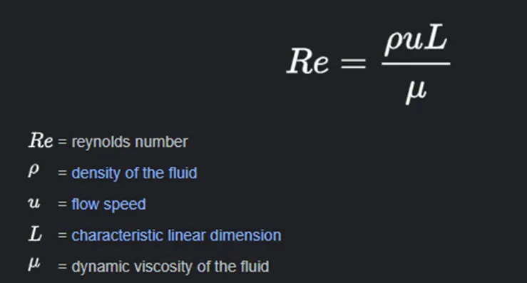
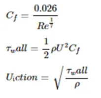
So, this are the formulas from we can calculate the Y+
After rearranging we got del y1
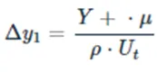
So Cf is the skin friction factor, Tw all is shear stress, Ut is frictional velocity.
So, this are the formulas and from these we got the values for all the 1st layer thickness
We got,
Re= 1794952.9171789 which is a turbulent flow
Cf=0.0033230525
Tw=1.272106035
Ut=1.0190455859
So, after putting all these values for different Y+ value we get different first layer thickness. we calculate the total layer thickness from the given formula
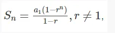
So, we got all things and calculate all the required values from the formulas, now we are going to see our meshes case by case,
CASE 1:
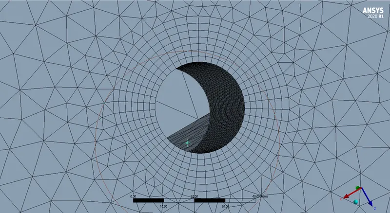
So, case 1 is very basic case because we use default settings of mesh to prepare this case although the results were very course so the element size for large encloser is 440mm also the element size for the small encloser is 440mm but the Ahmed body cylindrical support is 3mm. having inflation layer no. 6 and total layer thickness is 7.71561mm
The no. of nodes are50579, and no. of elements are 161309. The images of this case’s mesh are given below:
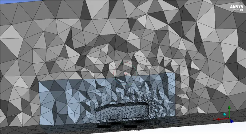
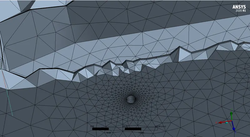
So, we can see that the case is not that much refined.
CASE 2:
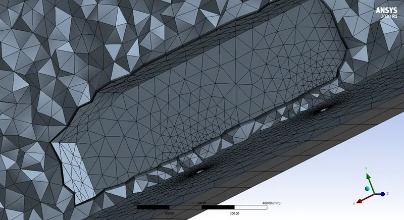
So, things got different from this case as this case cover Y + value of 70, having inflation layer 7 and total layer thickness 9.519464343814mm as the large encloser’s element size is 120mm and small encloser’s element size is 60mm with the element size of body’s support 3mm.
The no. of nodes is 66548 and no. of elements are 173923
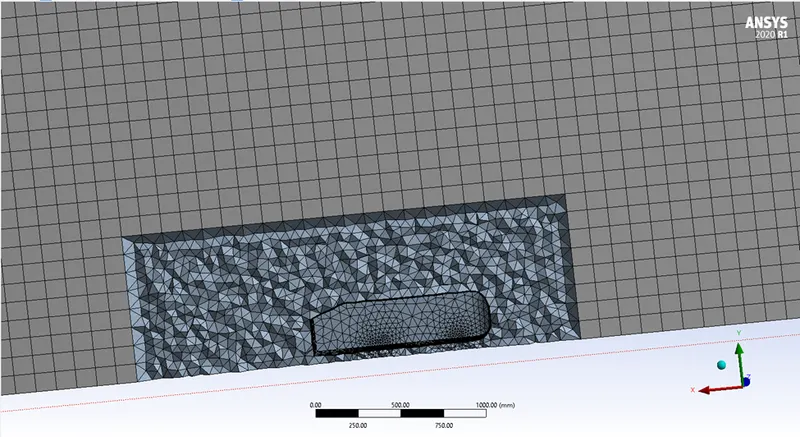
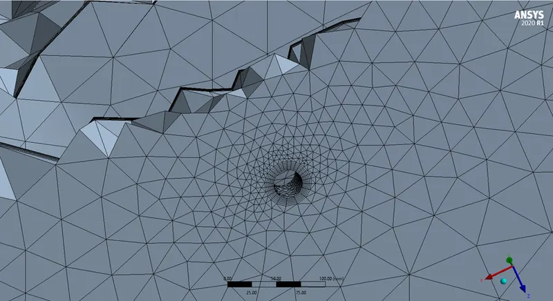
CASE 3:
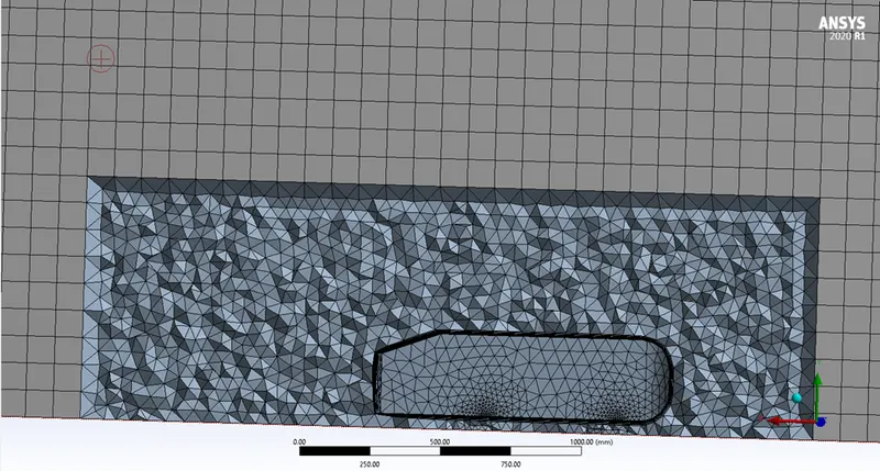
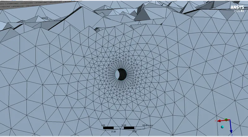
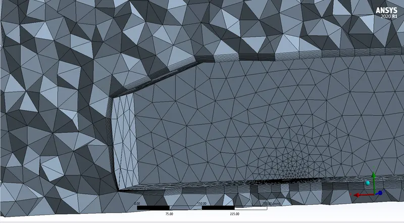
This case cover Y + value of 110, having inflation layer 8 and total layer thickness 18.0318510486mm as the large encloser’s element size is 100mm and small encloser’s element size is 50mm with the element size of body’s support 3mm.
The no. of nodes is 99144 and no. of elements are 259428 the images of mesh are shown as below:
CASE 4:
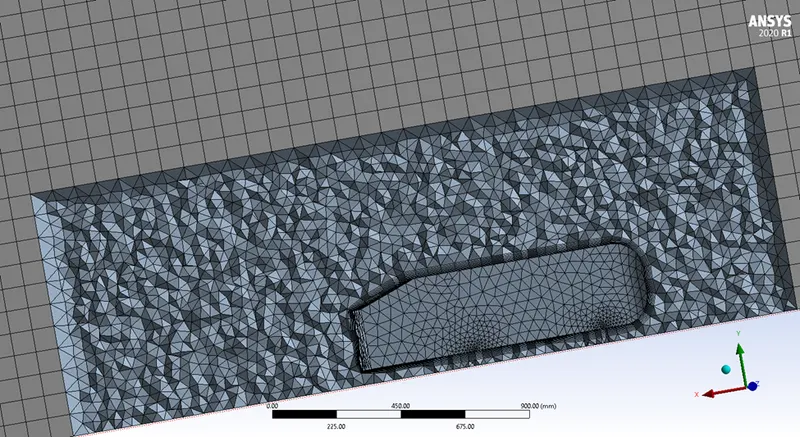
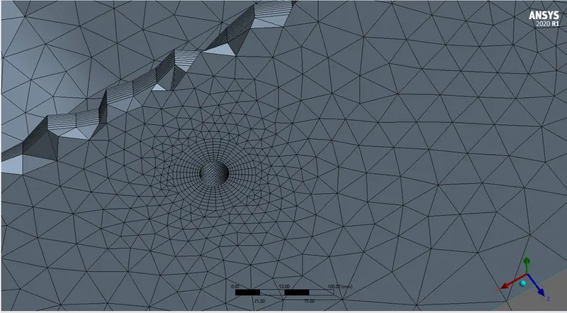
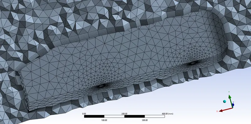
This case cover Y + value of 160, having inflation layer 9 and total layer thickness 31.1444569639mm as the large encloser’s element size is 80mm and small encloser’s element size is 40mm with the element size of body’s support 3mm.
The no. of nodes is 151124 and no. of elements are 399968 the images of mesh are shown as below:
CASE 5:
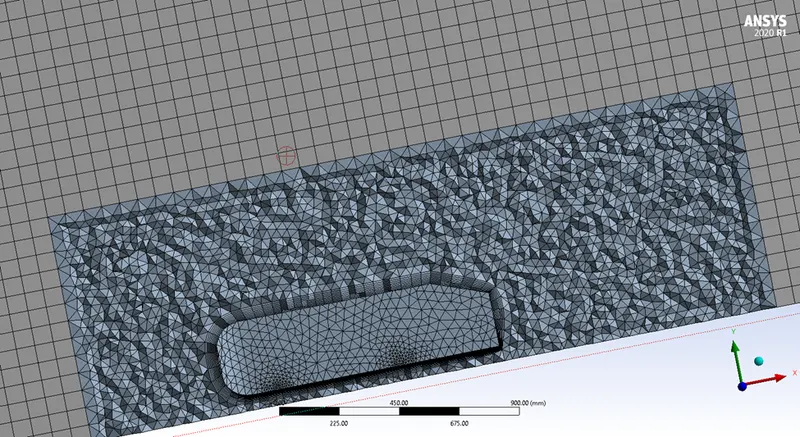
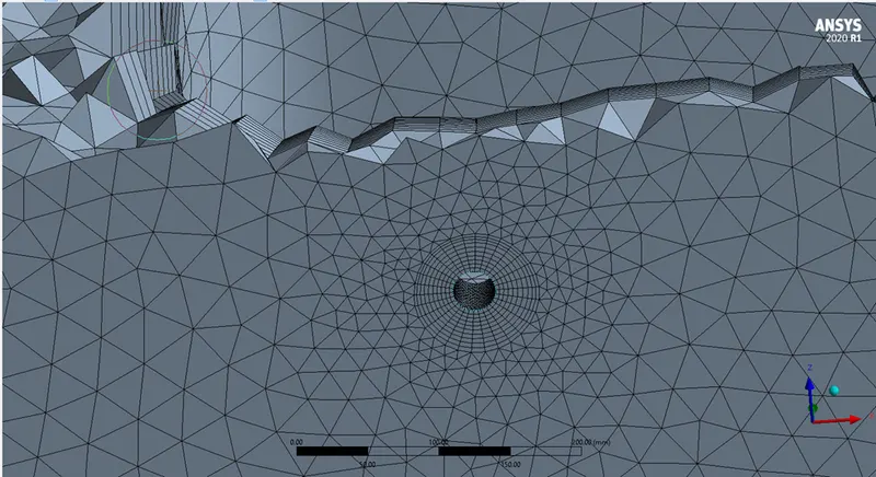
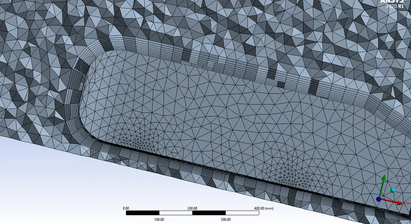
This case cover Y + value of 220, having inflation layer 10 and total layer thickness 50.2595450376mm as the large encloser’s element size is 70mm and small encloser’s element size is 35mm with the element size of body’s support 3mm.
The no. of nodes is 202057 and no. of elements are 547132 the images of mesh are shown as below:
CASE6:
This case cover Y + value of 270, having inflation layer 11 and total layer thickness 71.720658857mm as the large encloser’s element size is 60mm and small encloser’s element size is 25mm with the element size of body’s support 3mm.
The no. of nodes is 372307 and no. of elements are 1207315 the images of mesh are shown as below:
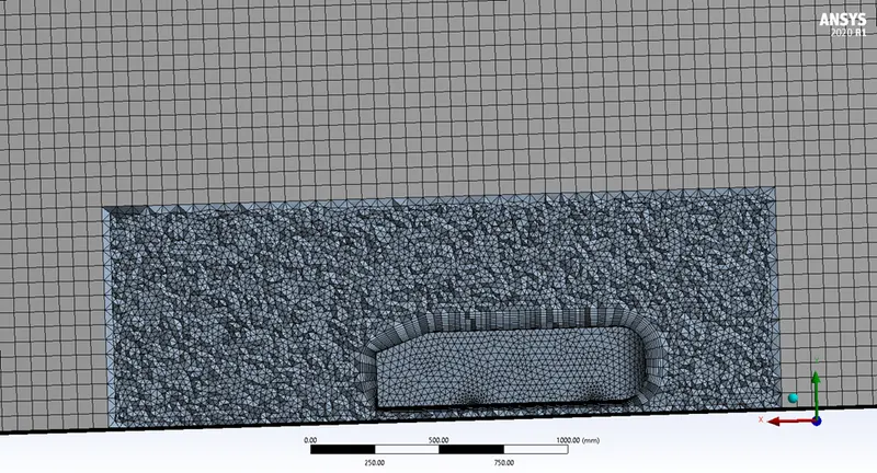
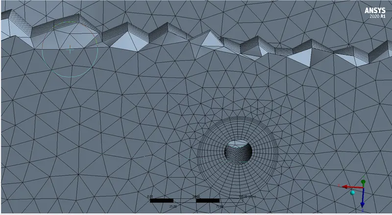
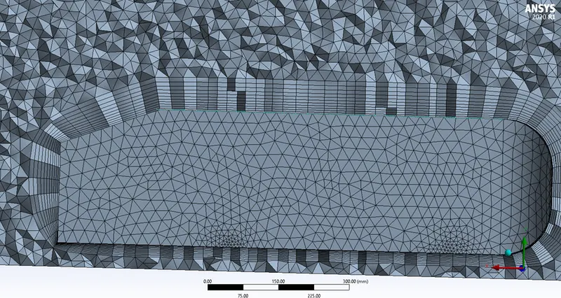
As we can see as we move case by case the mesh quality also improves.
CASE7:
This is most refined case which take a lot of computational power to run as the results were also amazing, this case cover Y + value of 290, having inflation layer 7 and total layer thickness 39.4377749243mm as the large encloser’s element size is 60mm and small encloser’s element size is 15mm with the element size of body’s support 2mm.
The no. of nodes is 969087 and no. of elements are 4596187 the images of mesh are shown as below:
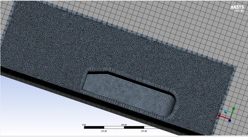
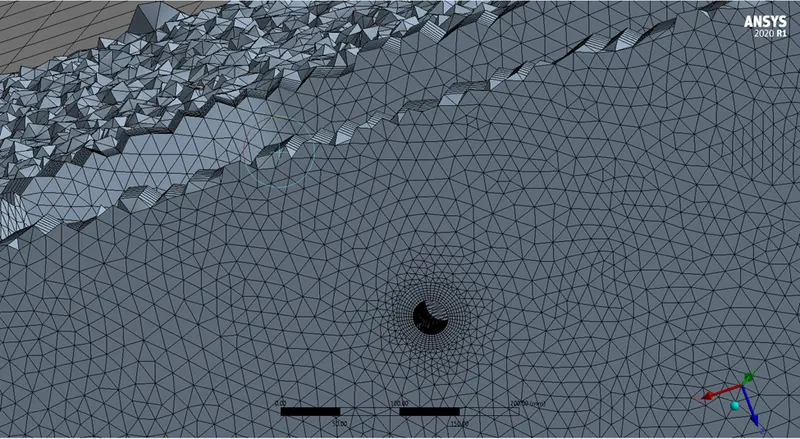
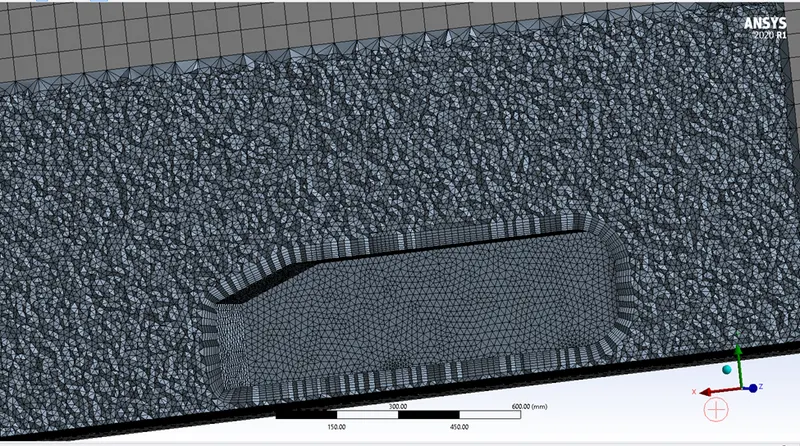
RESULTS:
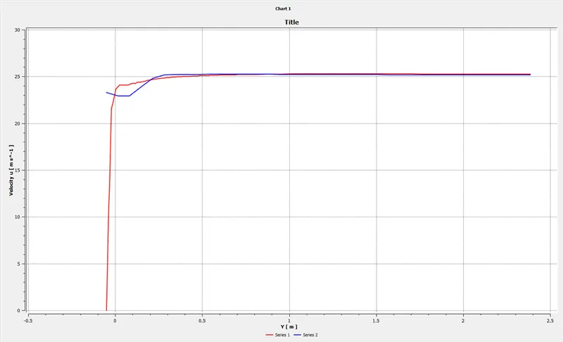
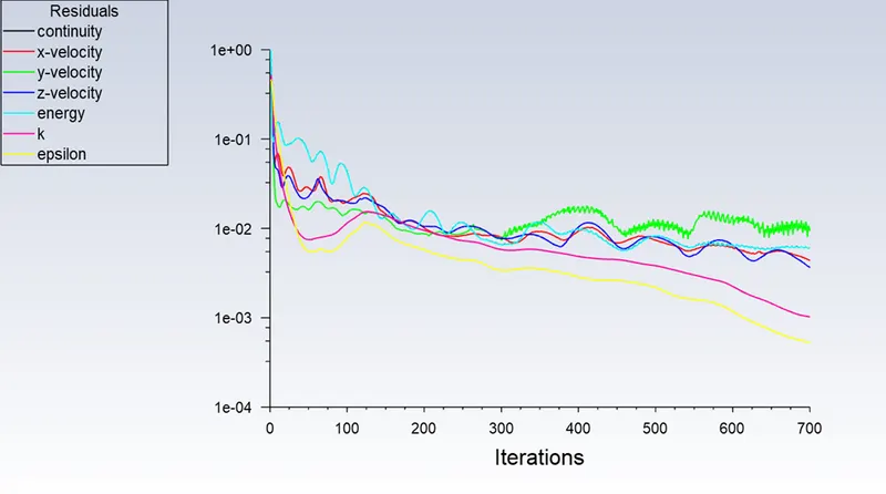
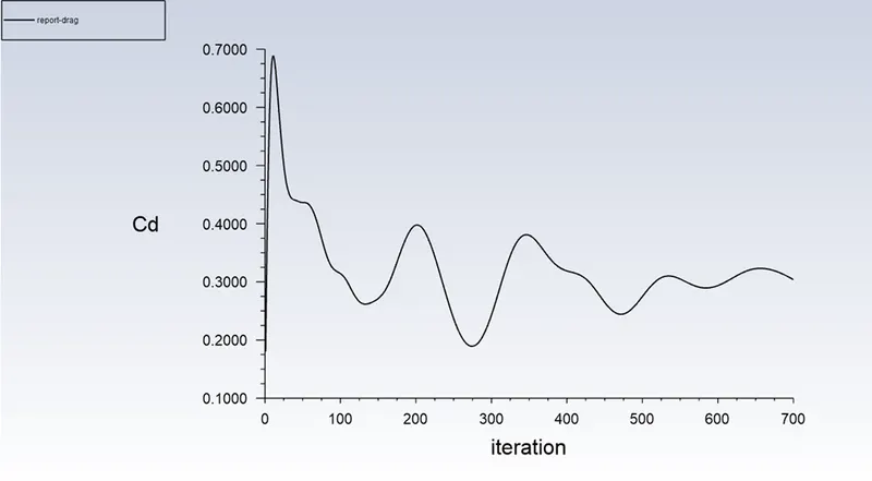
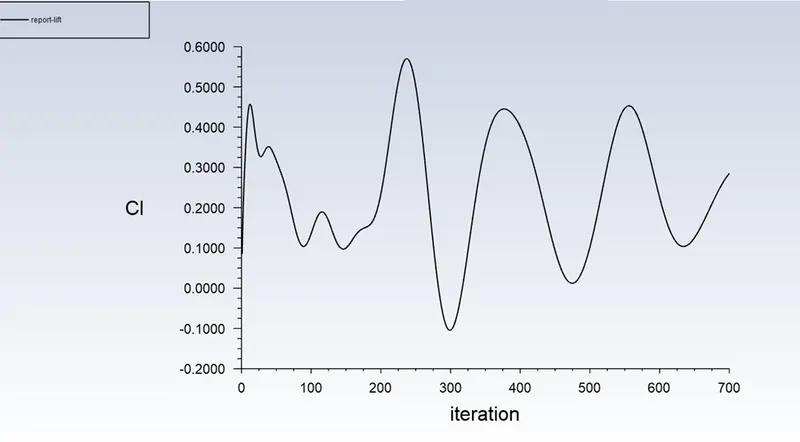
All the preparations are done all mesh are ready now we have to run each and every case in fluent so that we get our required answers that is contour plots for pressure and velocity, plot for drag and lift coefficient, vector for pressure and velocity, plot for residuals and the graph of u velocity-y .for the plot u velocity-y we have to create two line with two different coordinate on the velocity and then prepare the chart .so we start from the case 1
CASE 1:
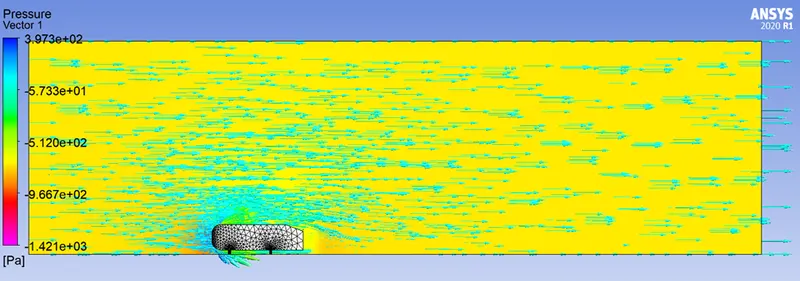
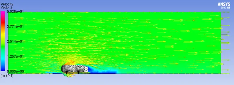
We can clearly see that the results from this case is very course
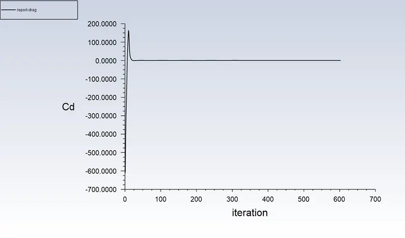
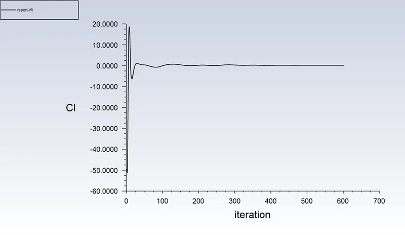
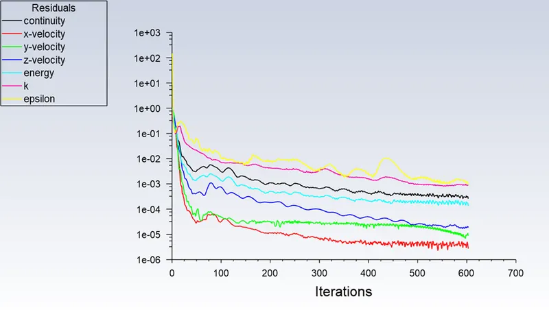
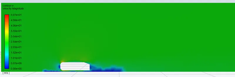
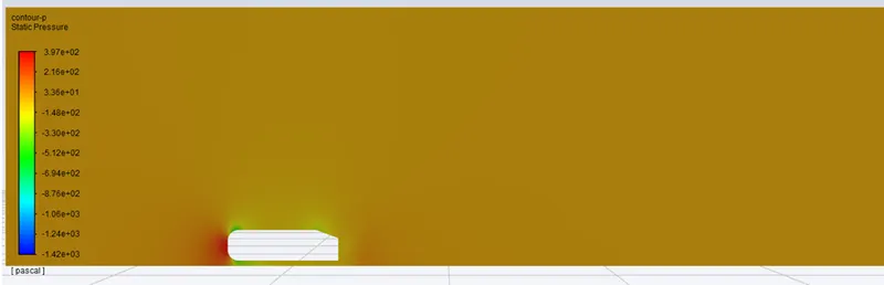
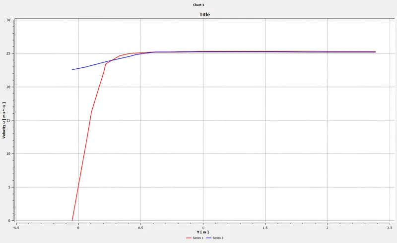
Hence the maximum u velocity is 2.53e+01
Cd=0.33072992 (0.2211878788% error)
Cl=0.20941706
CASE2: so, from here all the cases will be more fine
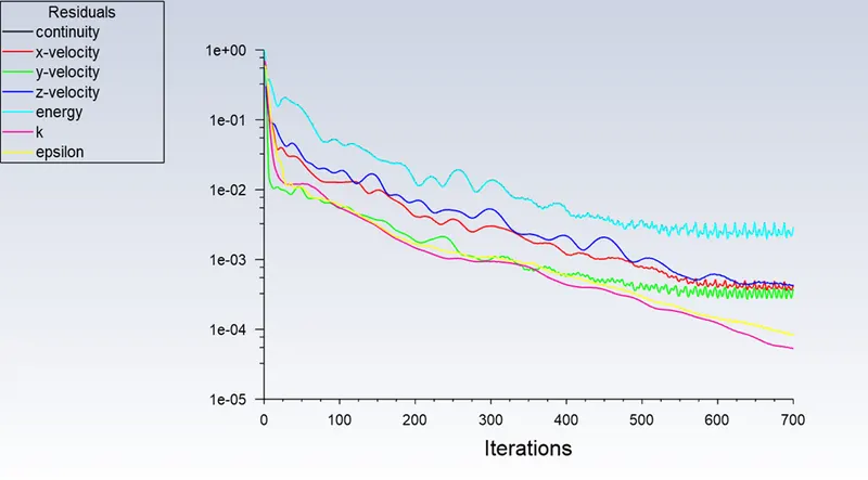
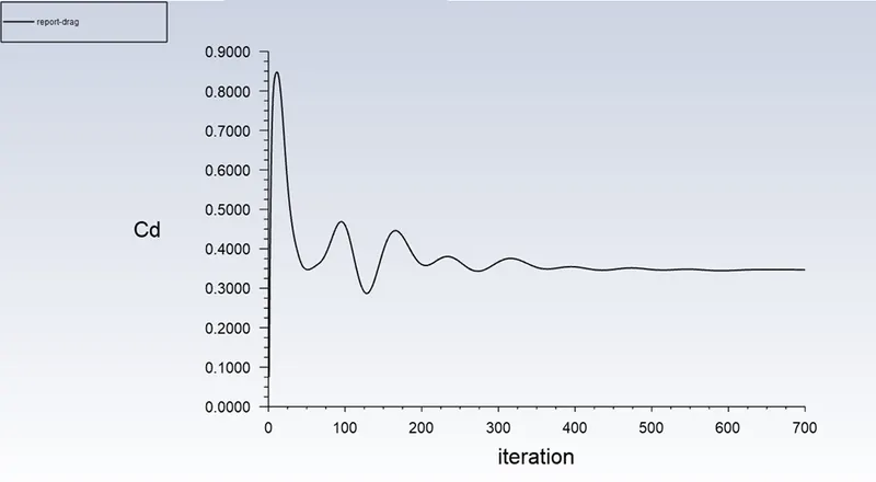
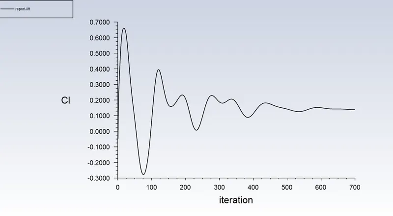
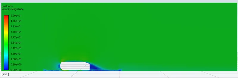
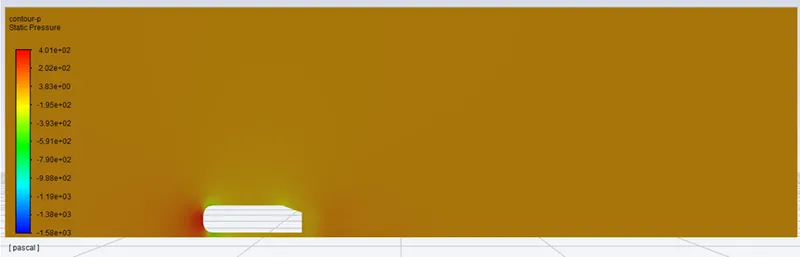
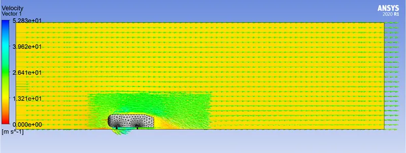
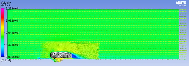
When we have a better mesh the no. of vector in small encloser increases. hence shows more fine results
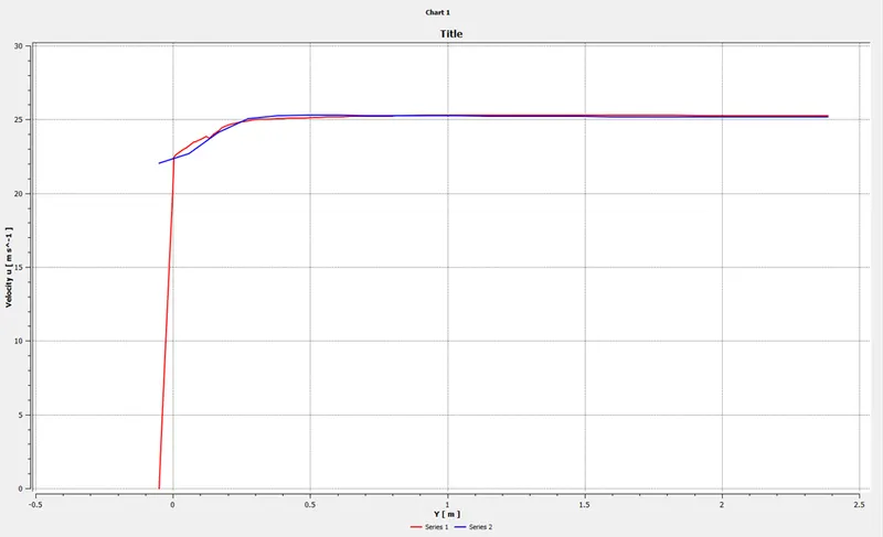
The maximum u velocity is 2.53e+01
Cd= 0.34676401 (5.0727%error)
Cl= 0.13821252
CASE 3:
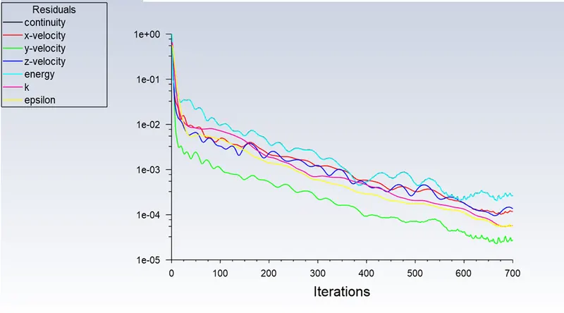
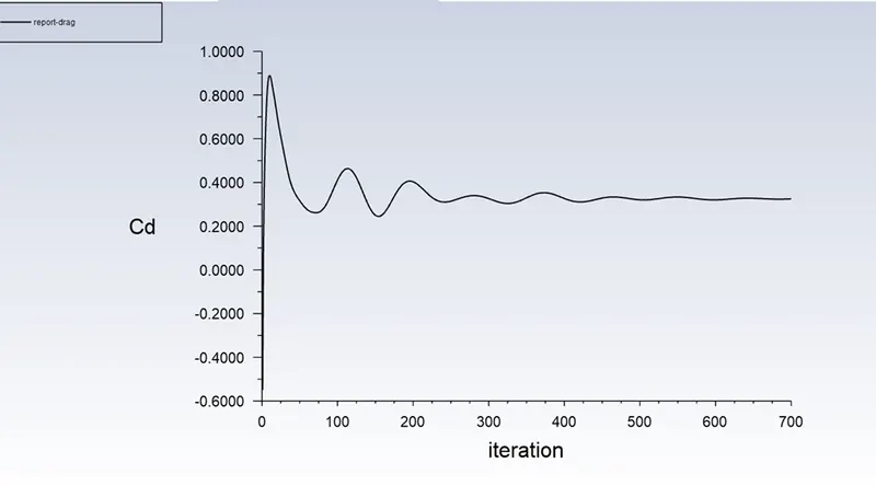
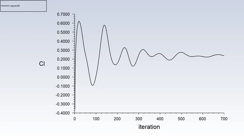
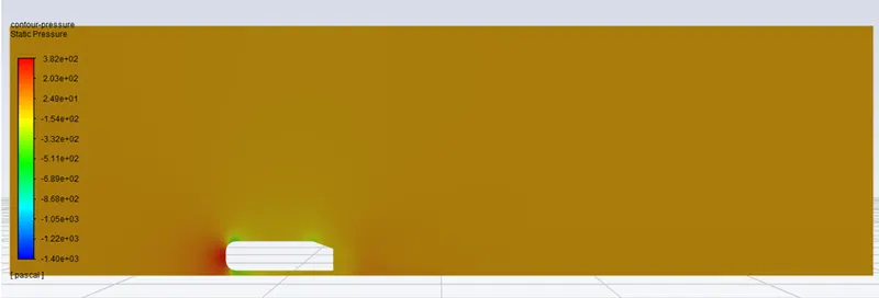
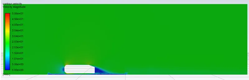
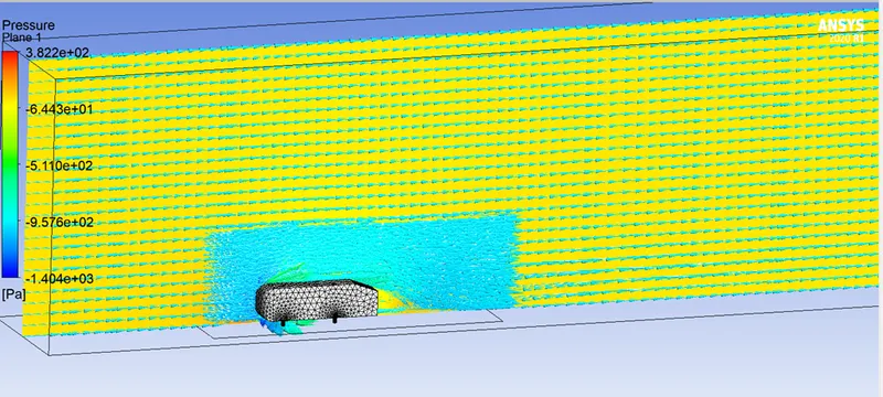
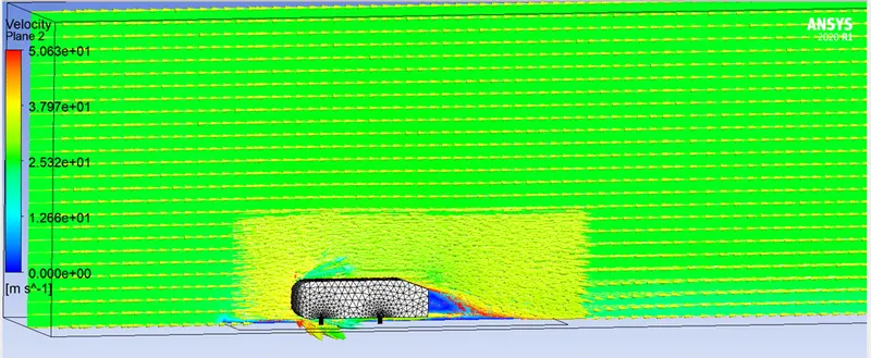
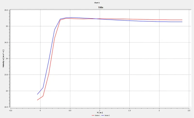
Hence in this case the maximum U velocity is 2.53e+01
Cd= 0.32472457 (1.5986151515%error)
Cl= 0.23708404
CASE 4:
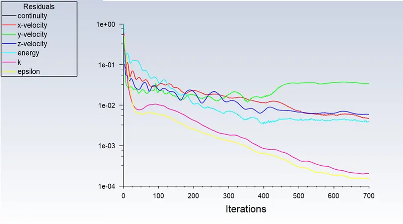
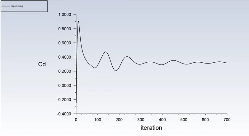
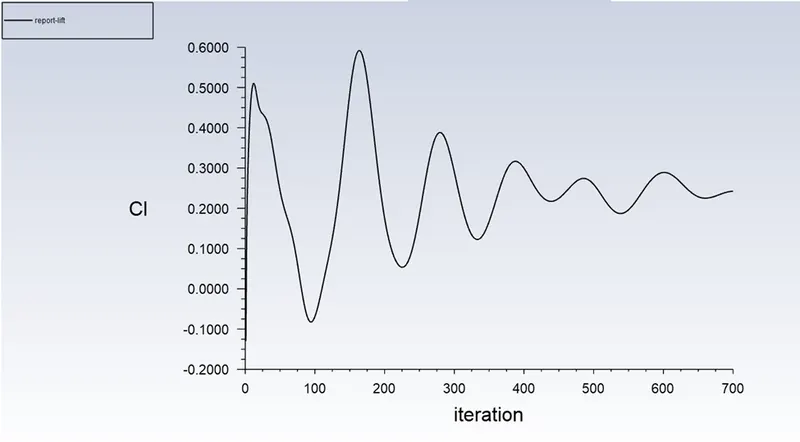
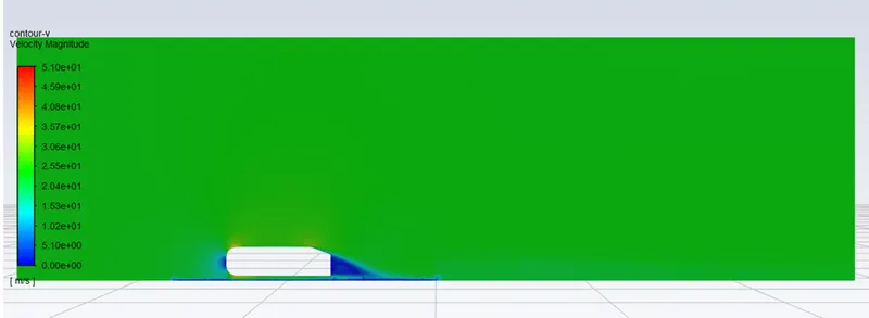
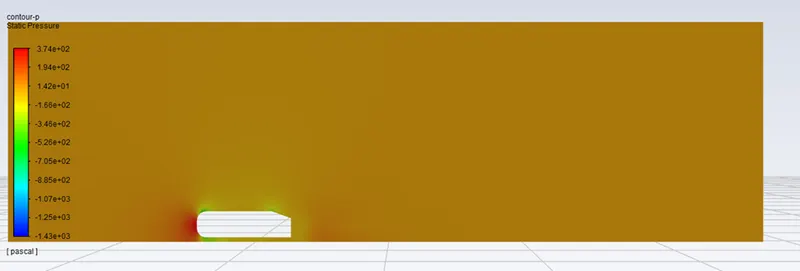
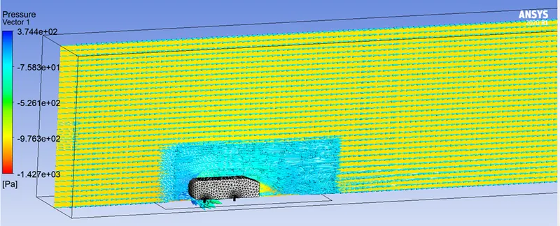
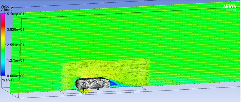
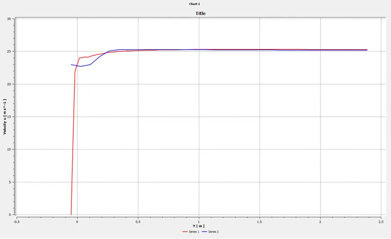
the max u velocity is 2.53e+01
Cd= 0.31530064 (4.4543515152%error)
Cl= 0.24249812
CASE 5:
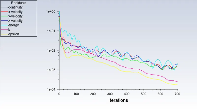
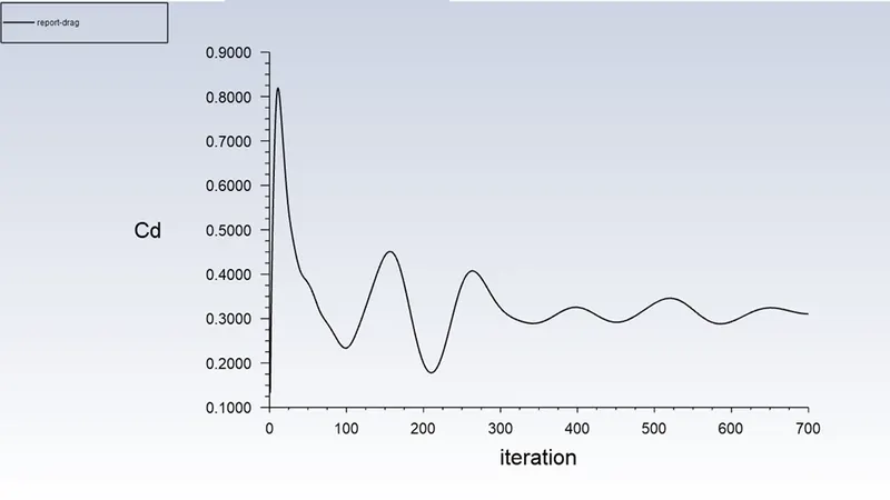
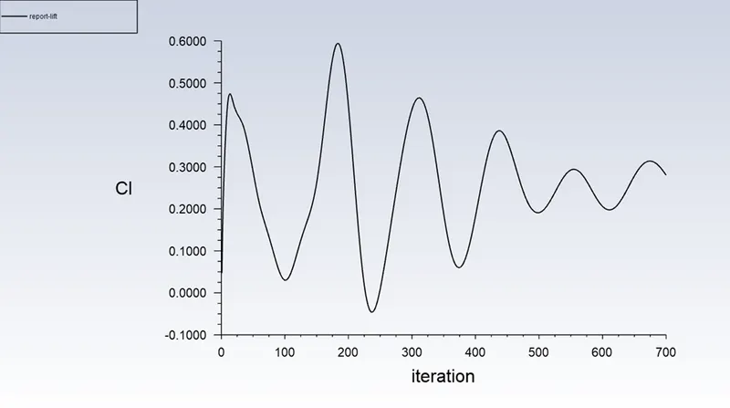
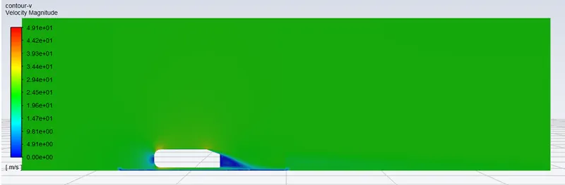
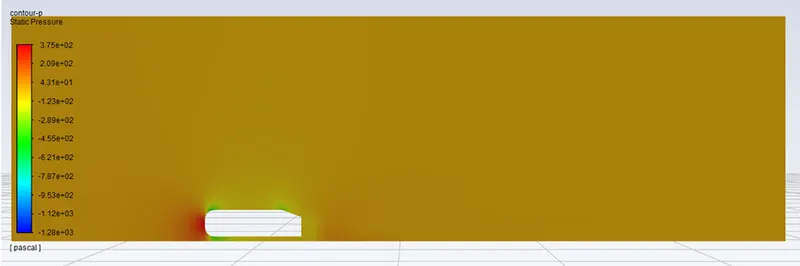
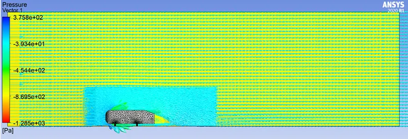
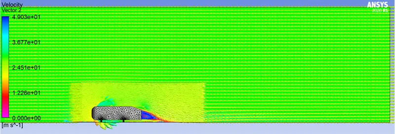
The max u velocity for this case is 2.53e+01
Cd= 0.31064533 (5.86520515152%error)
Cl= 0.2799021
CASE 6:
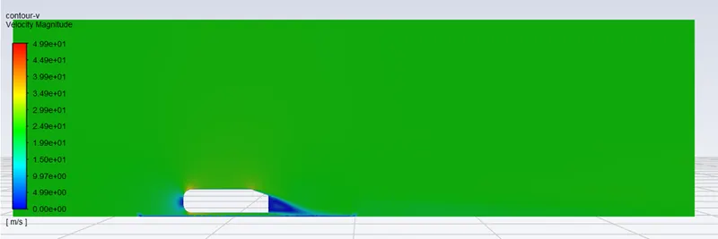
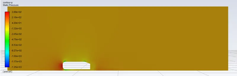
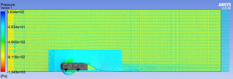
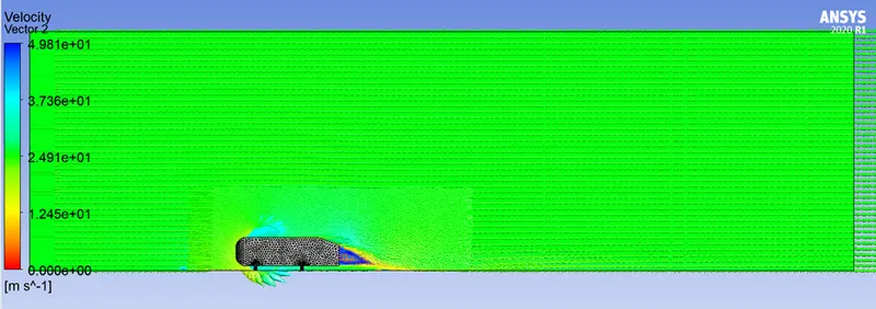
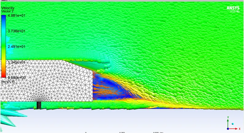
This is the recirculation Zone but this mesh is not fine so that we are not able to see it clearly.
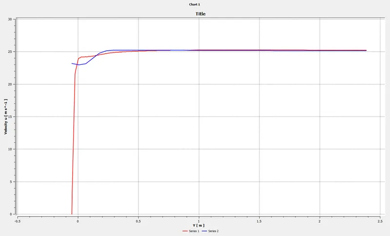
The max u velocity is 2.53e+01
Cd= 0.30374581 (7.96% error if we calc. it from 0.33)
(8.4806464286% error if we calculate it from 0.283 (reference value))
Cl= 0.28513752
CASE 7:
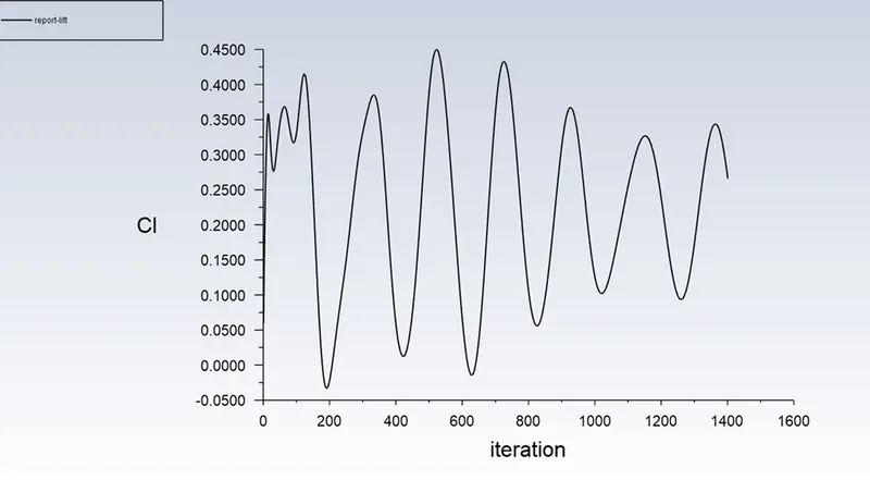
This case is the most refined case also the no. of iterations for calculating this case is 1400 rather then others its 2x more.
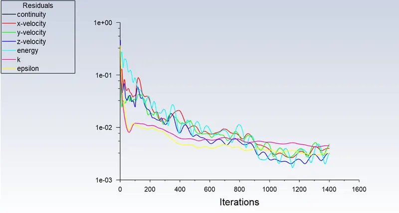
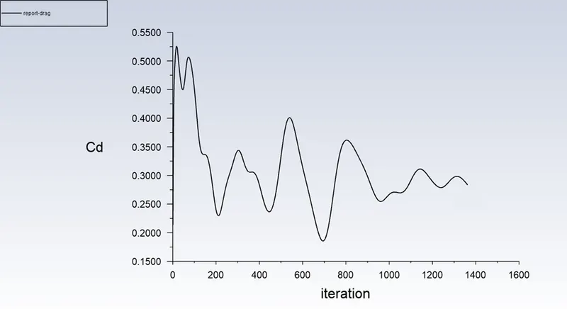
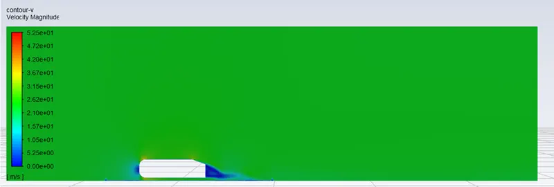
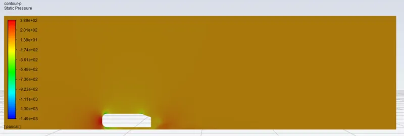
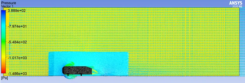
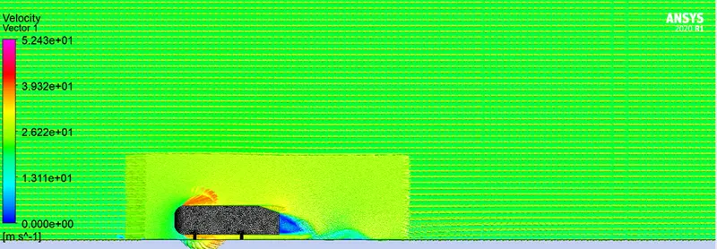
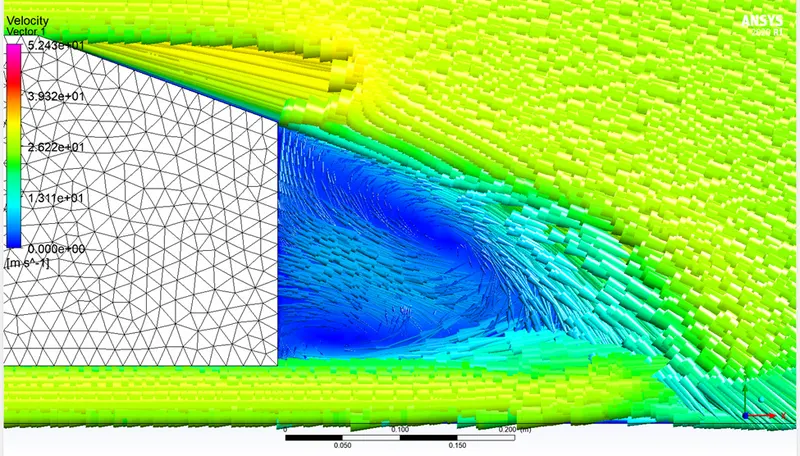
So here we can see that the mesh quality is far finer then the last case so that we can see the recirculation zone easily also in animation we are able to see the movement of the street formed behind the body moves as a vortex street but it was not as much big compared to the cylinder body case.
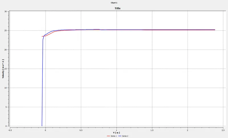
From series 1 max U velocity is 2.52E+01
And from series 2 max U velocity is 2.53E+01
Cd=0.26779312 (4.3596%error if we take the reference drag coefficient value 0.28)
Cl= 0.26589015
Negative pressure gradient: when fluid velocity increases the pressure decreases, hence there is an adverse pressure in the rear cause the boundary layer to separate out from the body and form the wake region, the formation of wake region take place when the wall shear stress and velocity becomes zero. These wakes are nothing but small vortices that create the negative pressure, this creates the circulation of velocity (shown clearly in case 7) and induce drag force. Hence the for the point of separation, it occurs due to an adverse pressure gradient encountered as the flow expands, causes a extended region of separated flow, as the flow goes farther downstream eventually it achieves a state of equilibrium which has no reverse flow. When the boundary layer separates, the remnants from shear layer and the present separated flow region b/w the shear layer and surface, modifies the outside potential and pressure field.
|
No. of case |
cd |
Cd % error with reference to 0.33 |
cl |
|
1 |
0.33072992 |
0.2211878788% |
0.20941706 |
|
2 |
0.34676401 |
5.0727% |
0.13821252 |
|
3 |
0.32472457 |
1.5986151515% |
0.23708404 |
|
4 |
0.31530064 |
4.4543515152% |
0.24249812 |
|
5 |
0.31064535 |
5.86520515152% |
0.2799021 |
|
6 |
0.30374581 |
7.96% with reference to 0.33 |
0.285135752 |
|
7 |
0.26779312 |
4.3596% with reference to 0.298 |
0.26589015 |
So in case 3 has more stable Y+ value because it has the minimum error percentage in drag coefficient
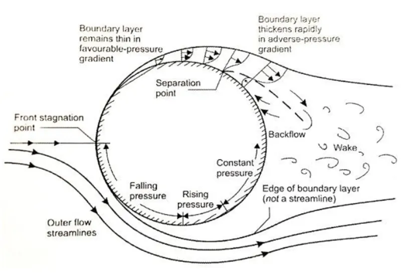
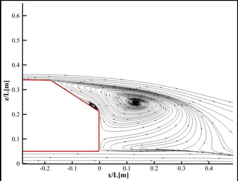
these are to show the wake region , recircuilating zone and point separartion
CONCLUSIONS:
- For the base mesh, case 1 we can see there is no proper wake formation as the results was far coarse then the required although if we put every reference value correctly the answer of drag coefficient is very close to the actual answer
- Wake formation can be seen I every fine mesh
- The grid independency test shown best results, with refining the mesh size with y+ factor the error the reduces for the predictive stable range as from the cases when we choose unstable one the value has more error percentage, as every drag coefficient try to achieve the reference value of 0.283.
- The recirculation zone and little vortex street can be seen clearly in the case 7 due to the refined mesh. Also, as mesh become more refined, we are able to capture flow more clearly as there is no proper wake formation in case 1.
- Higher &+ takes a lot time to be converged but still we will not be able to converge it completely
REFERENCE: