Week 1- Mixing Tee

AIM: To compare the mixing effectiveness with respect to different length and different inlets velocity in mixing tee using ANSYS fluent.

INTRODUCTION: We have to use ANSYS fluent to check the effective mixing of 2 fluids at different velocities also have to compare the k omega and k epsilon modals with a particular case and have to check which gives us better mixing animations. Also, we have to compare the effect of length over the mixing of the fluids and for a particular case we have to check if the mesh quality has any effect over the results.

THEORY: Mixing tees utilizes a specifically engineered internal geometry to efficient mix two fluids stream into one combined stream. So, we have a mixing tee, it has two inlets and have one outlet. From one inlet hot air will come and for another inlet the cold air will come, we have to check the effectiveness of mixing within the walls that how both the fluids will mix and give us the required temperature. These are widely used in the petrochemical, HVAC industry, etc.

SOLVING AND MODELLING APPROACH:

So, we have two type of geometries one is long tee and another is short tee, my analysis starts from the short tee and first I decide to choose the k-omega model for my analysis.

As I choose the k omega model and complete my analysis at default mesh settings and have the velocity and temperature for inlet on x axis (36degree C and 3m/s) and on y axis (19degree C and 6m/s) I got the average weighted temperature of approx. 33.600degree C. After that I choose the k-epsilon model for the same conditions and got more better results approx. 30.250degree C. Also, it is completely shown by the final results that mixing in k-epsilon model is much better than k-omega so for my further analysis I choose the k-epsilon model.

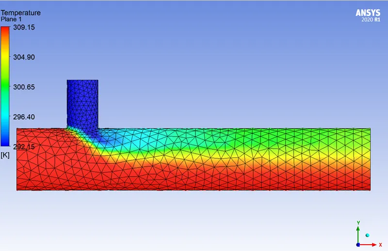
Results after using k-omega model, as we see the mixing at the outlet is not good.

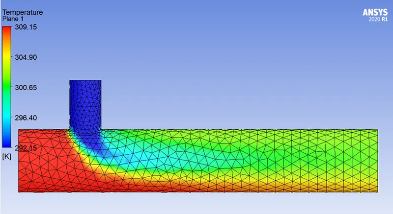
Results after using k-epsilon model, as we see that the mixing is much better then the k-omega modal.

After choosing which modal I choose I start my analysis over short tee modal with different velocity at inlet on y axis. So, we have constant temperature and velocty at inlet on x axis (36degree C and 3m/s) also have constant temperature at inlet on y axis (19degree C) then I divide this in two cases one in which we have different velocity at inlet.y axis (i.e 6m/s and 12m/s) getting those results and found out that 12m/s case gives results similar to required results(27.500degree C).

After complete the analysis over short tee modal I do same analysis with the same conditions on long tee and further divide the case into two to calculate the effect of two diferent velocity over long tee and found out that there is like negligible effect of long tee. So that was my approach and I use follwing modals of short tee and long tee:

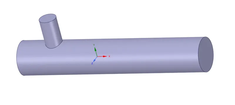
short tee modal

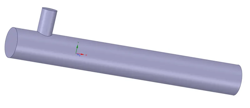
long tee modal

Also I analise long tee one more time with with more finer mesh that show me more good mixing in the tee although the results have negligible effect but we can see the effect of good mesh gave us good mixing.

PRE-PROCESSING AND SOLVER SETTING:

We have two modals of mixing tee one is long tee and another is short tee, following are some dimensions that we have to know:

SPECS	SHORT TEE	LONG TEE
Length from inlet.x axis to outlet of tee	0.1924m	0.2683m
Inlet.x daimeter	0.0339m	0.0339m
Inlet.y diameter	0.0170m	0.0170m
Area of tee	0.0237m^2	0.0318m^2

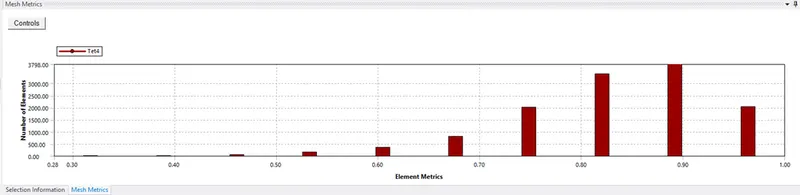
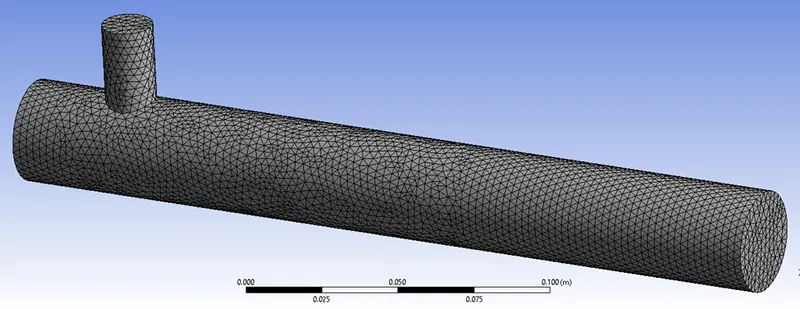
So after the geometry part we mesh the modal, I prepare 3 different mesh modals first I prepare the mesh modal of short tee with the default mesh settings , so it has 2797 nodes ,12583 elements and has the count of 12583 tetrahedral cells it looks like the following diagram:

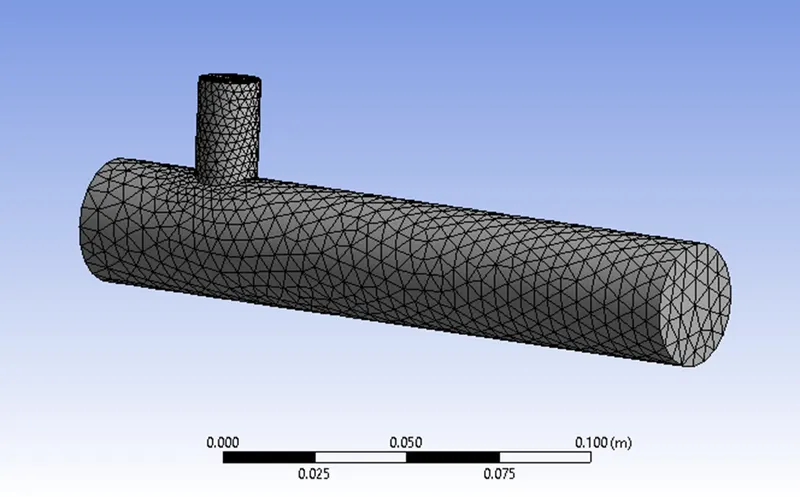
Also the elment quality plot is given below:

I also prepare the mesh moadal for long tee also and similar to short tee I use default mesh setting rather then more fine one , it has 3432 nodes,15368 elements and has the count of 15368 tetrahedral cells ,looks like the below diagram and also the element quality plot is below after the mesh modal:

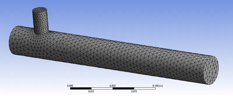
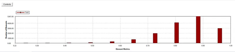
The third I prepare is of long tee with a adaptive setting of 7(maximum adaptive setting in ansys 2020 R1) having better mesh modal having 15839 nodes, 79430 elements and have a count of 79430 tetrahedral cells the diagram and element quality plot is given below:

Types of tee	No. of nodes	No. of elements	Cell count
Short tee with default mesh setting	2797	12583	12583
Long tee with default mesh setting	3432	15368	15368
Long tee with maximum adaptive mesh setting	15839	79430	79430

So, we are completely able to see the huge gap between the cell count also it affects the quality of mixing finer the mesh better we will able to see the mixing.

After the k-omega and k-epsilon difference I divided the analysis in 5 different cases

Sr. no.	cases
Case 1	Short tee having inlet.x axis velocity of 3m/s at temperature 36degree C and also having inlet.y axis velocity of 6m/s at 19degree C using default mesh setting
Case 2	Short tee having inlet.x axis velocity of 3m/s at temperature 36degree C and also having inlet.y axis velocity of 12m/s at 19degree C using default mesh setting
Case 3	Long tee having inlet.x axis velocity of 3m/s at temperature 36degree C and also having inlet.y axis velocity of 6m/s at 19degree C using default mesh setting
Case 4	Long tee having inlet.x axis velocity of 3m/s at temperature 36degree C and also having inlet.y axis velocity of 12m/s at 19degree C using default mesh setting
Case 5	Long tee having inlet.x axis velocity of 3m/s at temperature 36degree C and having inlet.y axis velocity of 12m/s at 19degree C using maximum adaptive mesh setting

Procedure:

Completeing our mesh model we go for setup and after that we choose the k-epsilon model and give the boundary conditions that I discuss in the table for each case after then we go for definition and give a surface report and go for two things area weighted average and standard deviation then give the no. of iterations that is required to check the convergence and see where we will be able to check the temperature at outlet. After then we will able to see the mixing in the tee(animation) with the help of cfd post.

RESULTS:

CASE1:

We have all things now we give all type of boundary conditions that are required and also have a good mesh now we’ll plot three types of graph for each and analyze the results

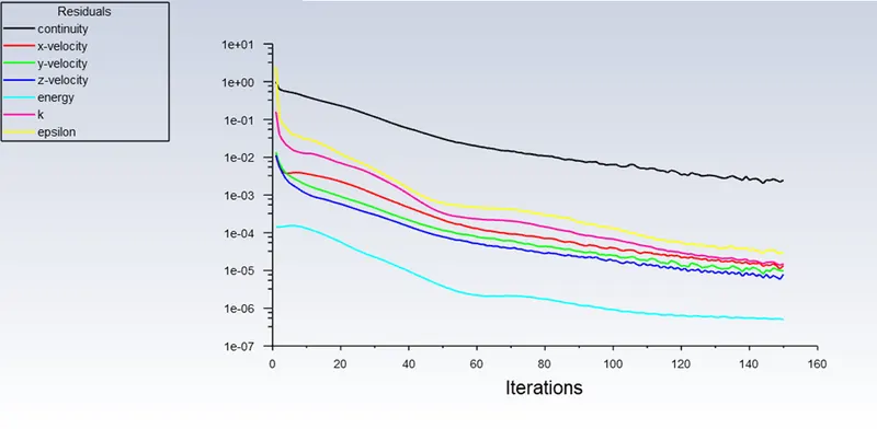
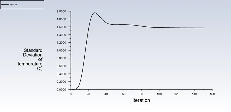
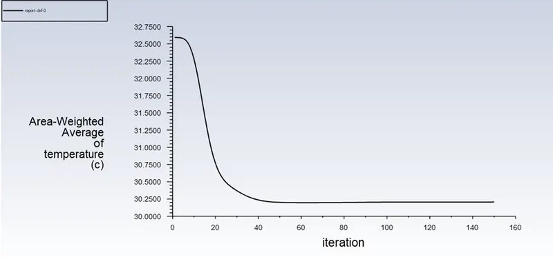
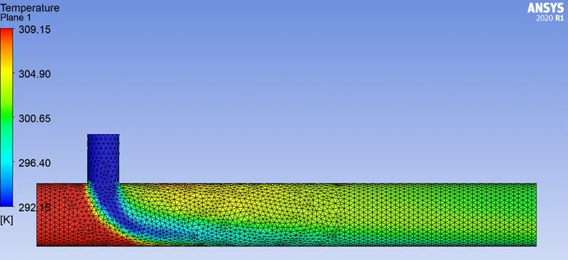
So from all these graphs we are able to see that in resiudals plot the no. of iterations are 40 because at 1e-05 is pretty good fpr convergence and also in standard deviation plot we can see that after 40 iterations the plot line is not that much disturbed and gives a value of approx 1600C and the main case of area weighted average of temperature also have convergence at 40 iterations and gives the value of 30.2500degree C. and the animation image might look like below image :

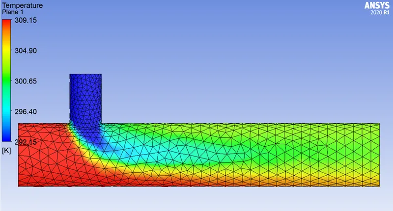
CASE2:

Similarly like above case we will calculate three type of graphs according to boundary condition this time the inlet.y axis is 12m/s double then 1^st case the plots are given below:

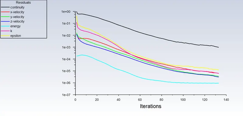
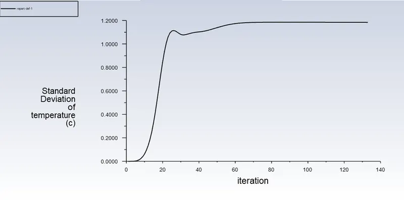
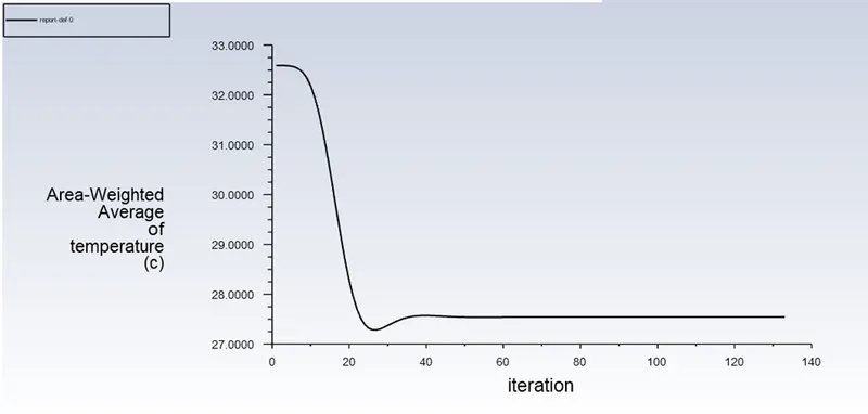
We can see the similar thing in the residual plot it comes gradually increasing to approach the zero the best no. for convergence is at 40 again we can see in area weighted average of temperature have convergence at 40 iterations and is gives a very near amount of required result answer i.e 27.500 degree C also the standard deviation convergence is between 40 to 50 and gives a value of 1100C and the animation image is given below:

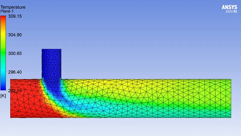
CASE3:

Bothe the cases above was of short tee and now we have case of long tee agin we will plot three graphs which are given below:

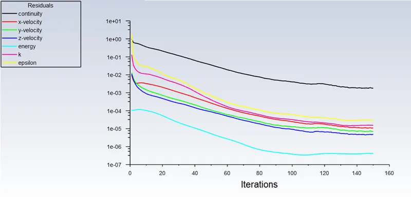
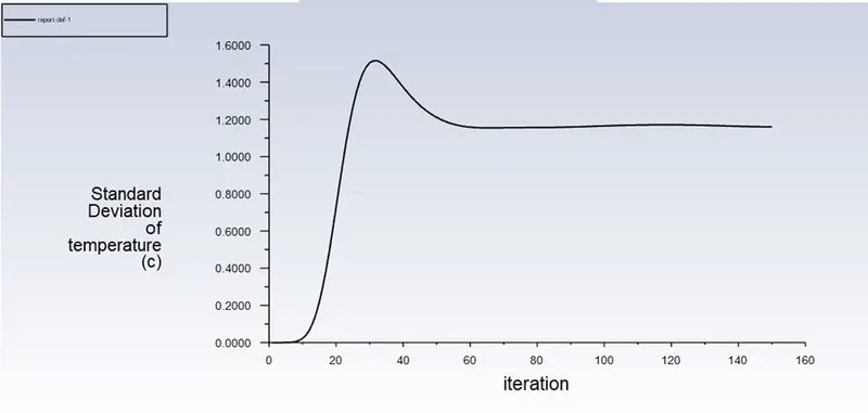
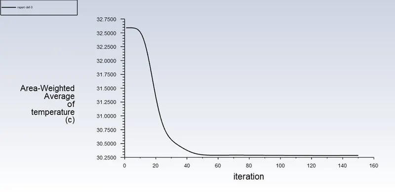
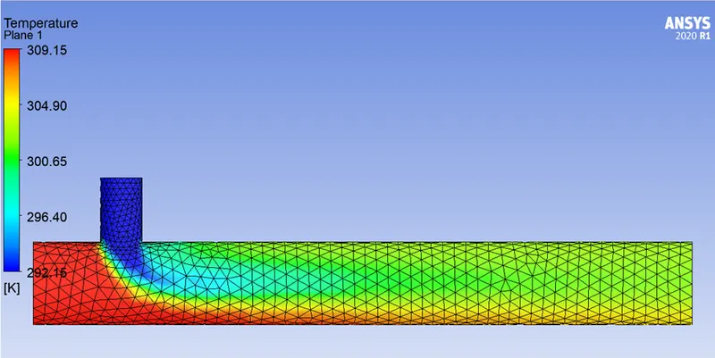
We can see thes time the no. of iterations for convergence is at 50 for all three graphs and area weighted average of temperature value is at approx 30.3715degree C. also it gives vaue approx of 1200C for standard deviation at 50 iterations.The result image is given below:

CASE4:

Similar case of long tee we have to plot three graphs similar to case 2 it has 12m/s velocity for inlet.y axis. The graph which we plot are given below:

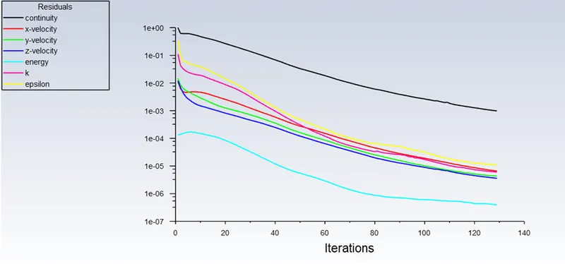
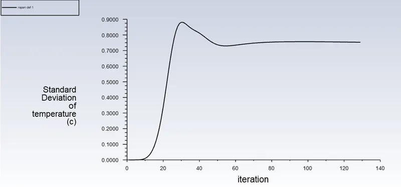
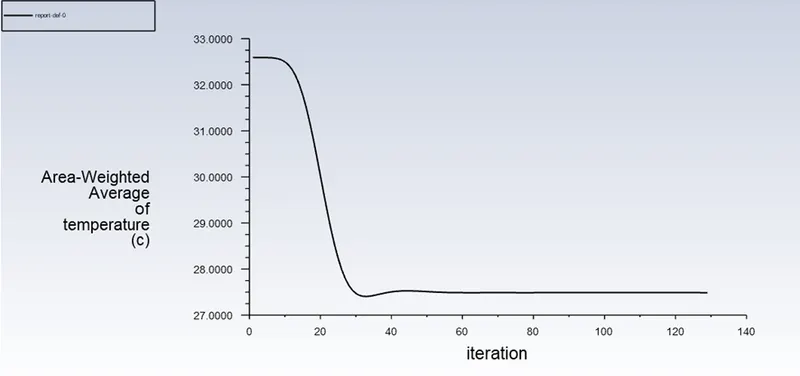
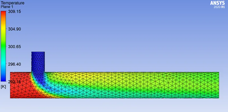
So here we can say that coveregence iteration in case of residual plot is 40, for standard deviation plot convergence iteration number is between 40 and 50 and gives value of 7250C and for area weighted average the convergence iterations is 40 gives us the temereature value of 27.1215degree C. Also the result are shown below from there we can see the mixing in tee:

CASE5:

It is the only case where we have better mesh quality then other cases ,similar to other cases we have to plot three graphs, those are given below:

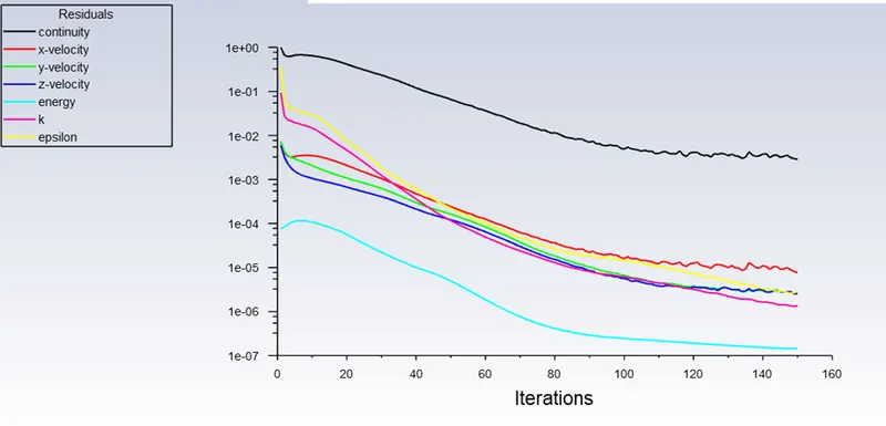
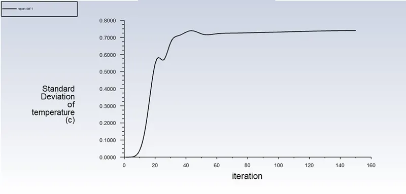
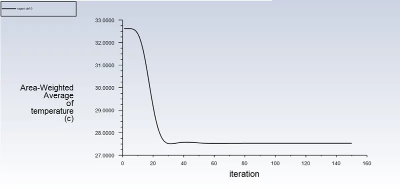
Hence the convergence no. 1e-05 the iterations are aprox 30 to 35 , also area average temperature it shows same iteration no. 30 to 35 and shows a value of 27.500 degree C and for standard deviation it shows convergence in between 40 to 45 gives a value of 7000C after that the plot line goes for satability.

Sr. no.	Average outlet temperature in C	No. of iterations for convergence
Case1	30.2500	40
Case2	27.5000	40
Case3	30.3715	50
Case4	27.1215	40
Case5	27.5000	35

CONCLUSION:

After completing all analysis we know some points that I discuss below:

• K-epsilon modal is much better then k-omega modal for mixing tee modal
• Velocity have a very huge impact in these cases to get the required temperature more the velocity from y axis inlet better will be result
• Better the mesh ,finer will be the mixing between two fluids
• Length does not affect the mixing and also does not helps us to get the required results