Week 2 - Flow over a Cylinder.

AIM: simulate the effect flow over a cylinder and explaining the phenomenon of vortex shedding with the help of average velocity plot, drag coefficient and lift coefficient plot.

INTRODUCTION: In fluid dynamics, vortex shedding is an oscillating flow that takes place when a fluid such as air or water flows past a bluff (opposing the streamline flow and having no slip condition) at certain velocity, depending on the size and shape of the body. In this flow, vortices are created at the backward of the body and detach periodically from either side of body forming a Von karman vortex street. The fluid flow past the object creates alternating low-pressure vortices on the downstream side of the object. The object will tend to move to low pressure zone. In ANSYS we can analysis how the vortex shedding looks like over some particular Reynolds no. with finer mesh so that we are able to see how actually the whole process works out with different different Reynolds no. and also, we will able to see the effect of Reynolds no. by comparing it with the drag coefficient, that how drag coefficient will change as we increase our Reynolds no.

THEORY: so first we just run our simulation for steady flow for re 100 and then also for unsteady and try to find the strouhal no. As for finding the strouhal no., we have to plot the lift coefficient and then we just have to plot the FFT plot to find the strouhal no. the mathematical expression to solve the strouhal no. is give below:

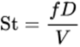
Where St is the dimensionless strouhal no., f is the vortex shedding frequency, D is the diameter of the cylinder and V is the flow velocity. And strouhal no. is only calculated for the unsteady flow (transient) because it depends on the frequency that can be calculated by the time factor or flow time only and only the transient modal will able to solve our problem with these factors whereas the steady flow is not able to solve our problem as we will see in further research that steady modal only counts the magnitude and no. of iterations only.

For calculating the strouhal no. and get a perfect value we have to change the quantities for a particular Reynolds no. so that we can have less error (by comparing the values with reference papers)

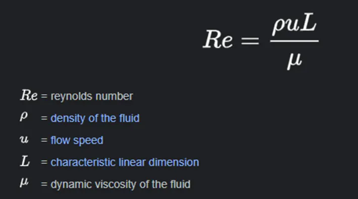
So, we just change the density, dynamic viscosity and flow speed to get our answers. Some of the application helps to construct the tall building, analyzing the turbocharger interaction with a pulsatile flow through time resolved flow measurement upstream and downstream of the turbine, combustion and mixing control for analysis of the advanced propulsion, flow measurement and many more.

SOLVING AND MODELLING APPROACH: first we made our geometry with the dimensions that I will discuss in preprocessing after that we just go for a finer mesh, the more the finer mesh the better will be results after that we just have to analyze our problem in 2 parts and run the simulation to get the converged plots and vortex shedding plot, also we have to create the monitor point at which we can plot our vertex average for velocity magnitude will be plotted we also create the animation so that we will see the effect completely

so, we have two parts for the analysis

part1: in this part we have to calculate the strouhal no. for re 100 for both steady and unsteady flow, in this part we will be able to show that the strouhal no. only be calculated for unsteady flow as the steady modal will not able to count the time factor.

We have reference empirical formula to calculate the vortex shedding

Strouhal's empirical formula for the frequency of vortex shedding is f = (1/5) (v/d)

we will able to calculate the frequency and then put the value in the Strouhal’s formula that we discussed above from these formulas we will be able to calculate it more perfectly also it is effective to choose the values for the velocity, viscosity and density so that we will get our desired results.

Part 2: where we have to calculate the coefficients of drag and lift over a cylinder by setting the Reynolds number to 10,100,1000,10000,100000 also have to plot the graphs of lift, drag coefficients and have an image of a diagram in which we can see the effect of vertex shedding.so for calculating and choosing the values we have formula for drag coefficient

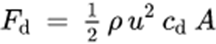
Here Fd is drag force, rho density, u velocity, A area and Cd is the coefficient of drag. So, all these formula helps us to get a more accurate value.

Also, we have to discuss the effect of Reynolds no. on coefficient of drag by comparing values and validating it to be in under 5% from the below image

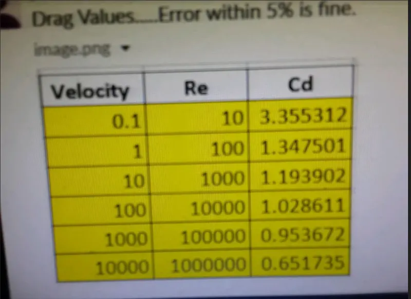
As the result of this question will be: with increasing the Reynolds no. drag coefficient decreases for that we have perform our analysis over different Reynolds no. and we will able to prove this point.

PRE-PROCESSING AND SOLVER SETTING: so now what we have idea what we have the problem so first we make a 2D modal in which can conduct our analysis

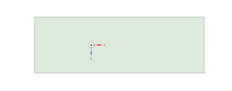
So, this our diagram the specs are, we have a cylinder of 2m diameter from the center of the cylinder to the inlet is 10*D length and the length from the center of the cylinder to outlet is 20*D and the distance between the symmetry walls is 20*D so we have rectangle like modal having area of 60*20 m^2. After designing our modal, then we also have to create the monitor point which we can create only in the results of fluent the monitor point will be 4*D m from the center of the cylinder and in the direction of +ve axis (outlet direction), we go for mesh

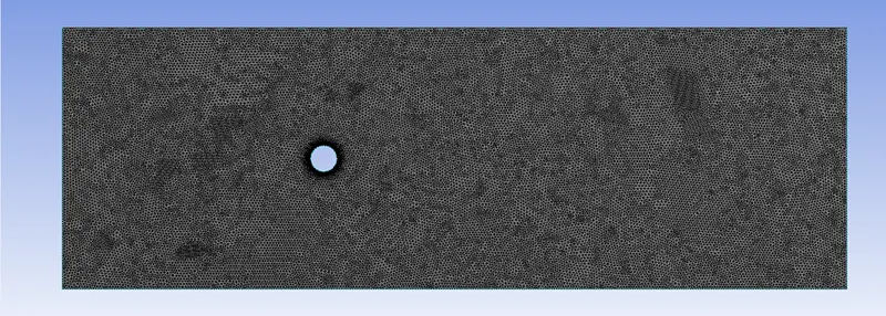
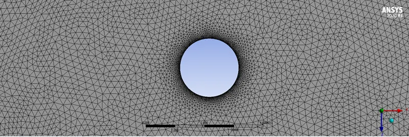
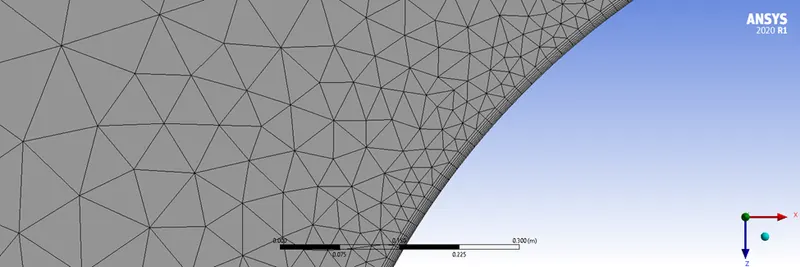
So, the mesh is having a triangle method, and have a sizing of 360 divisions for more finer results over the cylinder and in inflation we used the first layer thickness of 1E-003 m having maximum layer 7 and growth rate 1.2. also, the element size for each case the element size is 0.2 m that’s why we have this much finer mesh the no. of elements is 69218 and the no. of nodes are 36433.

After preparing our geometry and after performing the mesh, we will open our ANSYS fluent and have to perform our analysis like I describe it below:

PART 1:

1^st we will simply prepare two modals for steady and unsteady flow for re 100, after that for steady modal run the analysis for 1200 iterations and plot the drag coefficient, lift coefficient, vertex average and contours of our velocity magnitude.

Similarly, we run the for 2000 timesteps having a size of 0.1 s and we see that we got our drag coefficient, lift coefficient , vertex shedding and velocity contour for the cases then with the help of FFT we plot a graph strouhal no. then we able to see that for steady flow there is no plot because strouhal is based over frequency and frequency is based over time and steady modal will not able to plot the graph whereas the unsteady flow gives us the value of 0.16 (strouhal no.) also plot the graph for it.

For both the modal I used simple scheme solution method, and also run it in laminar flow in viscous modal.

Type of flow	Area (m^2)	Velocity (m/s)	Dynamic viscosity (kg/m s)	Density (Kg/m^3)
Steady	2	2	0.06	1.5
Unsteady	2	2	0.06	1.5

2^nd we run our simulation for re 10, 100, 1000, 10000, 100000 with the given values so that we can get very small error percent we plot graphs for lift, drag coefficients, vertex medium and contour for velocity and after that we can compare the drag coefficient with Reynolds no. and see the effect over the

body, analysis will be done in simple scheme solution method also we use the hybrid form the values for the analysis is given below:

Reynolds no.	Area (m^2)	Velocity (m/s)	Dynamic viscosity (kg/m s)	Density (Kg/m^3)
10	2	2	0.4	1
100	2	2	0.06	1.5
1000	2	100	0.3	1.5
10000	2	2000	0.6	1.5
100000	2	13500	0.54	2

So, these are the values which insert to get the minimum error for the drag coefficient, all the error percentages and the plot, convergence, contour will be covered in the result section.

RESULTS:

PART 1:

strouhal no. formula=(omega*L)/v

where omega is oscillation frequency, l is characteristic length and v is flow velocity

Case 1, when we have steady flow re 100: so, for this particular case we just plot some graphs like the residual, vertex medium for velocity magnitude, drag and lift coefficient and then try to solve the strouhal no. with the help of lift plot we prepare a FFT for strouhal no. as we plots are given below

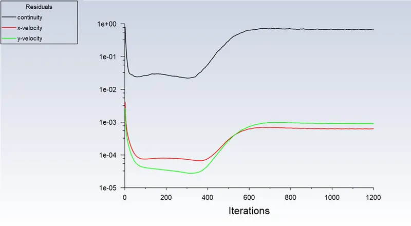
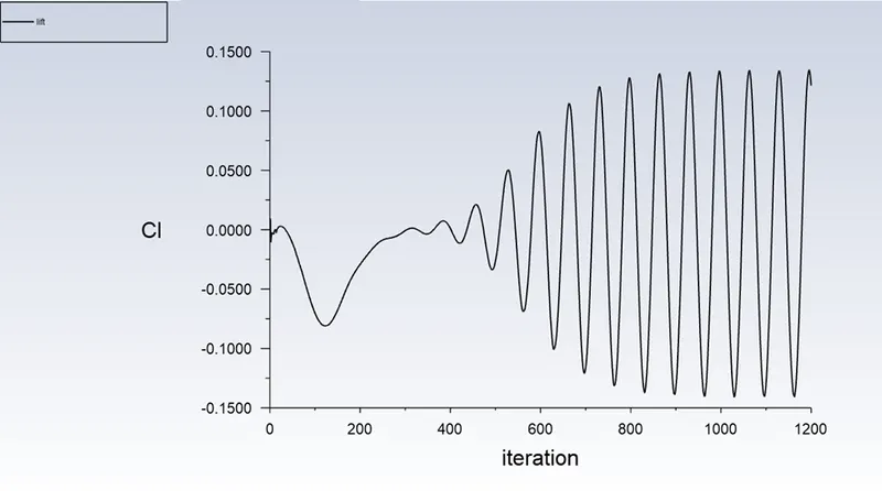
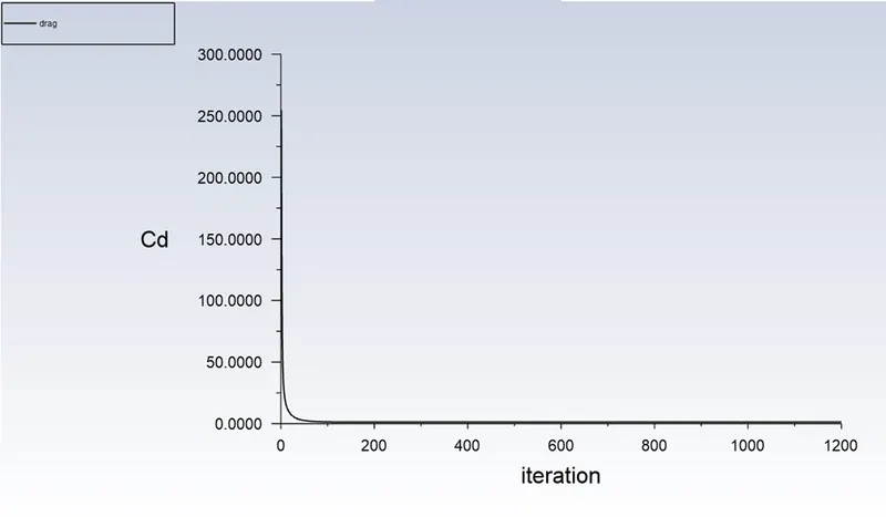
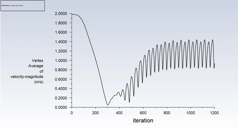
As we can see the residual plot is stabilize after 600 iterations and the vertex average and lift coefficient plot is converging at about 810 iterations, but we are not able to calculate the strouhal no. as we are not able to find the frequency so we can say that for steady flow we will not be solve the strouhal value as steady state records the activities as the flow gets stable, there is no time factor consideration take place.

Cd= 1.3593551 (0.8797099223% error)

Cl=0.12145854

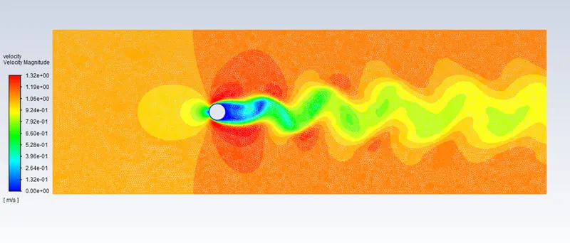
Case 2, when we have unsteady flow re 100:so, for the unsteady flow we use the transient modal because in this modal the activities of flow recorded starting from t=0. so first I will show the plot for the residual as given below:

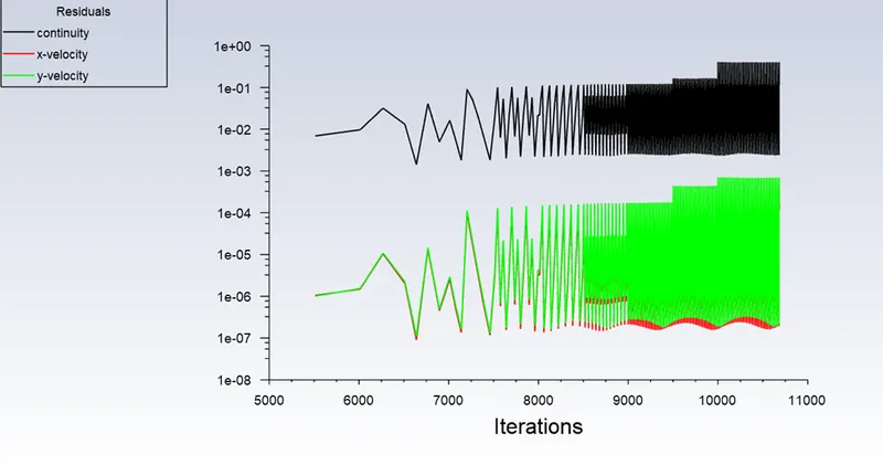
So, this plot shows that residuals are stabilizing after 9000 iterations as the pattern it shows now is similar to the final plot that we get after 40000

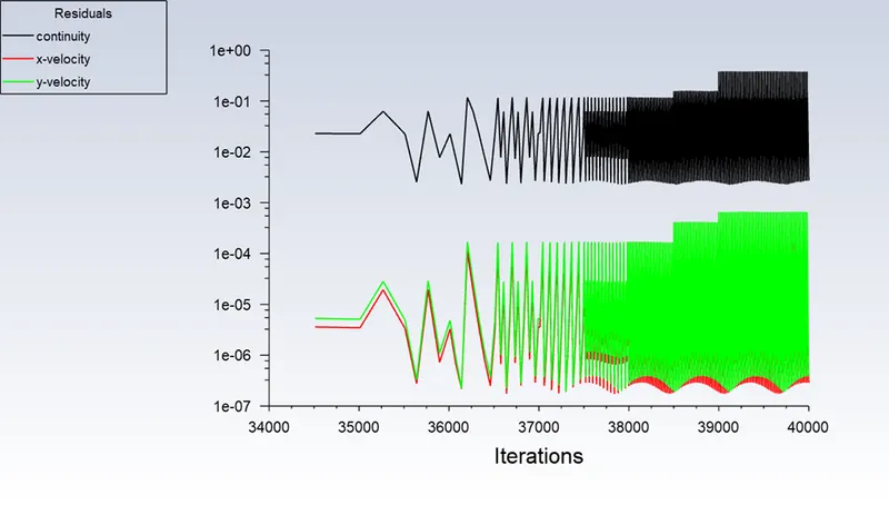
After that we will see the other plots, contour and also solve the strouhal no.

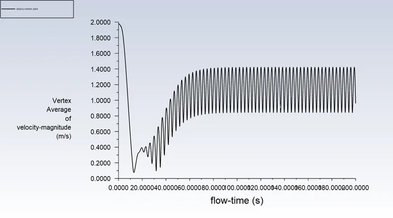
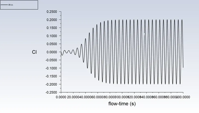
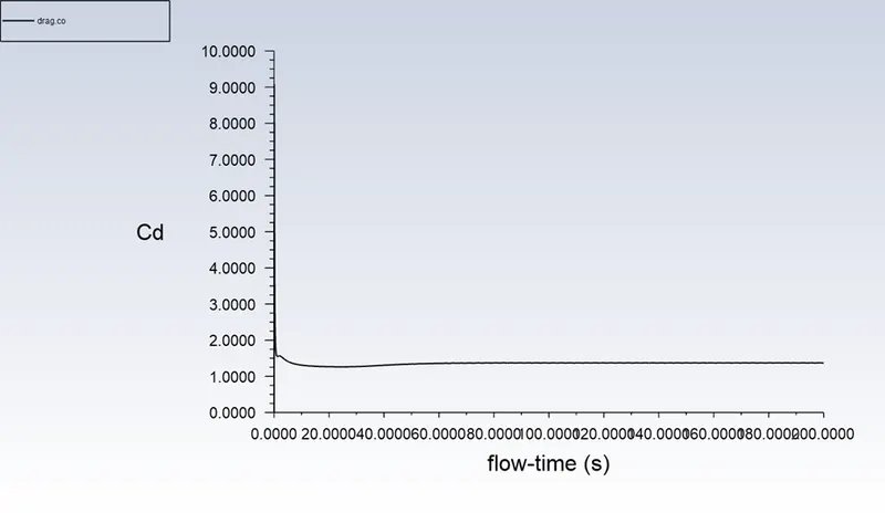
So, we from these plots we are simply can see that after 80 iterations our plots are getting converge from these plots, we will also prepare a FFT plot for strouhal no. also the lift and drag coefficient with pressure and velocity contour are given below:

Cd=1.3715489(1.7846294734%error)

Cl=0.18011875

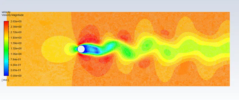
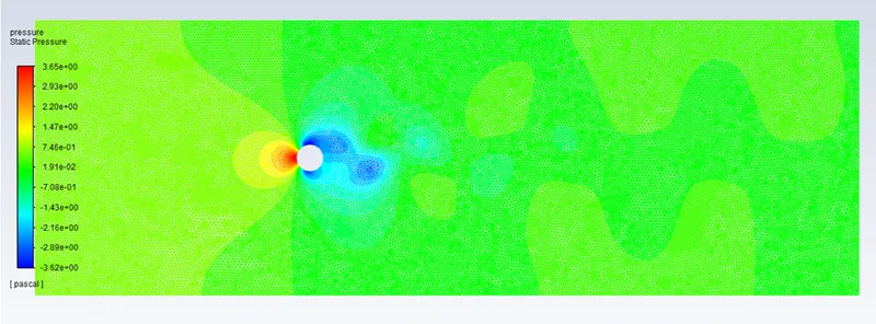
As from the strouhal formula we can see that there are approx. 8 oscillations in between the flow time of 50s (100-150 = 8 oscillations)

So, from the omega formula we get= 8/50 which is equal to 0.16 and if we put these value in strouhal no. we get

St= (omega*L)/v

So, for this case L is 2m and v is 2m/s so,

St= (0.16*2)/2

St= 0.16

Also, the plot for strouhal no. is given below:

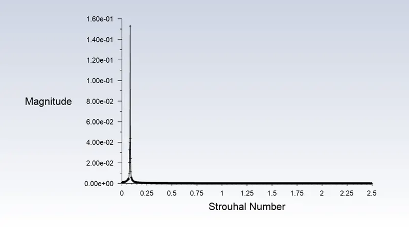
Strouhal no. for re 100 unsteady flow is 0.16

PART 2:

CASE 1, when we have Reynolds no. 10: so, for re 10 I run fluent for 1600 iterations but there is no vertex shedding (I also calculate for 4000 iterations)

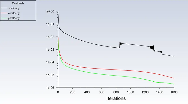
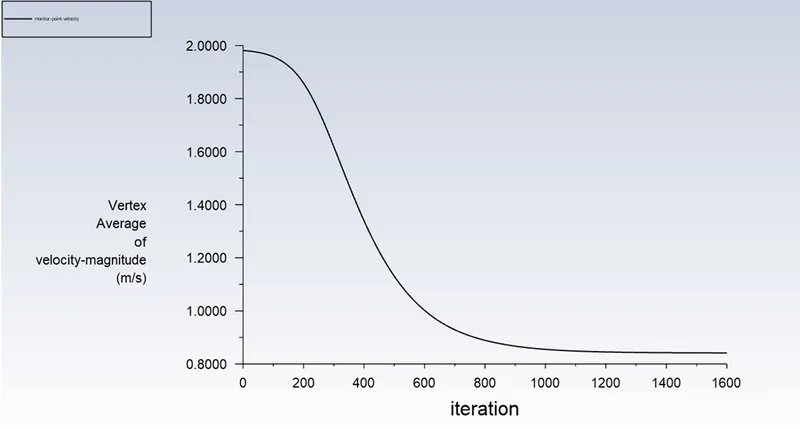
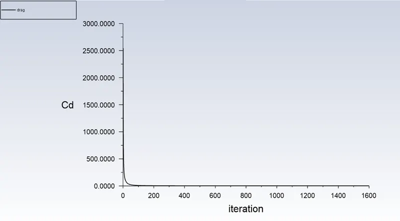
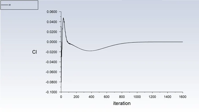
So, there is convergence after 900 iterations in vertex medium but re 10 does not show any type of vortex shedding also the lift and drag coefficient are given below:

Cd=3.3397778 (0.462973339%error)

Cl= -0.0003237437

Also, the contour for the velocity is below this:

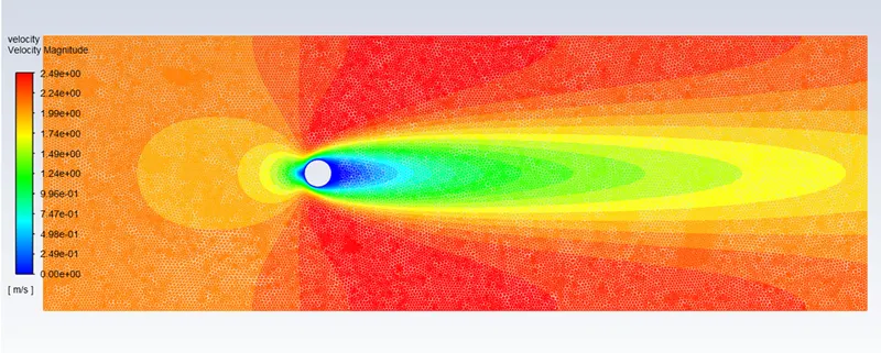
CASE 2, when we have REYNOLDS NO. 100: now for re 100 I run the fluent for 1200 iterations after that we got our required plots and the values of drag coefficient, the plot and contours for the re 100 are given below:

So, we are able to see that after about 600 iterations our residual plot start stabilizing.

So, from the above plots we conclude that after approx. 810 iterations our vertex medium and lift coefficient starts converging as we see there is no more fluctuations after 810 iterations also the drag and lift coefficient are

Cd= 1.3593551 (0.8797099223% error)

Cl=0.12145854

Vortex shedding is look like below image:

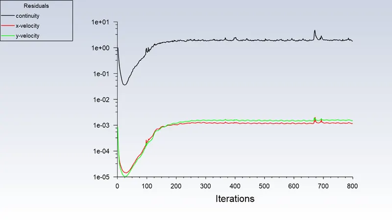
CASE 3, when we have REYNOLDS NO. 1000: so, for re 100 we can see that after 250 iterations residual plot is stable

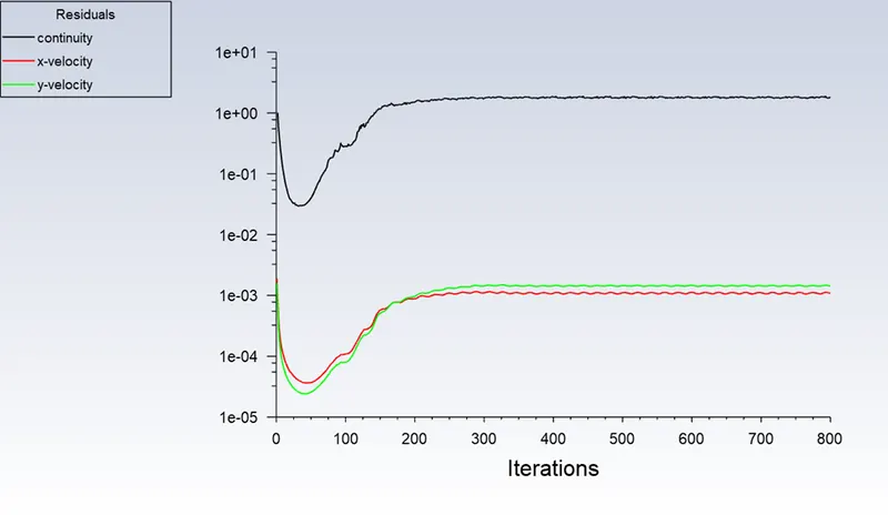
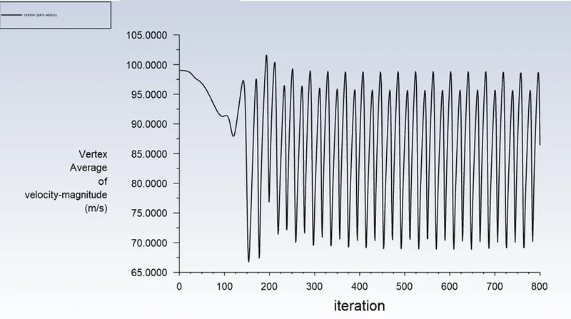
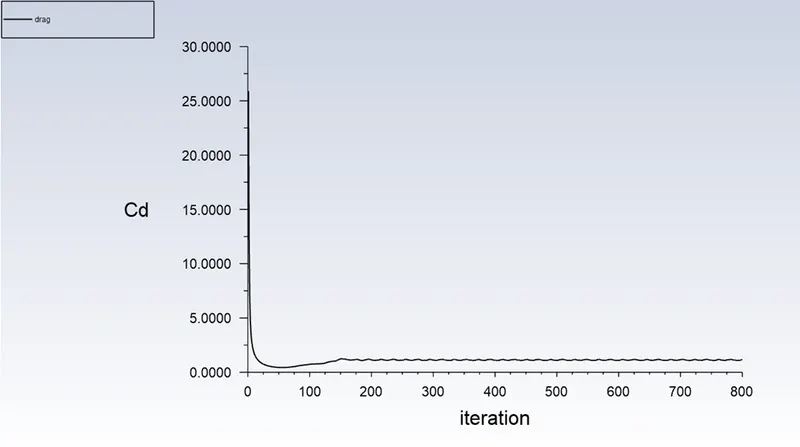
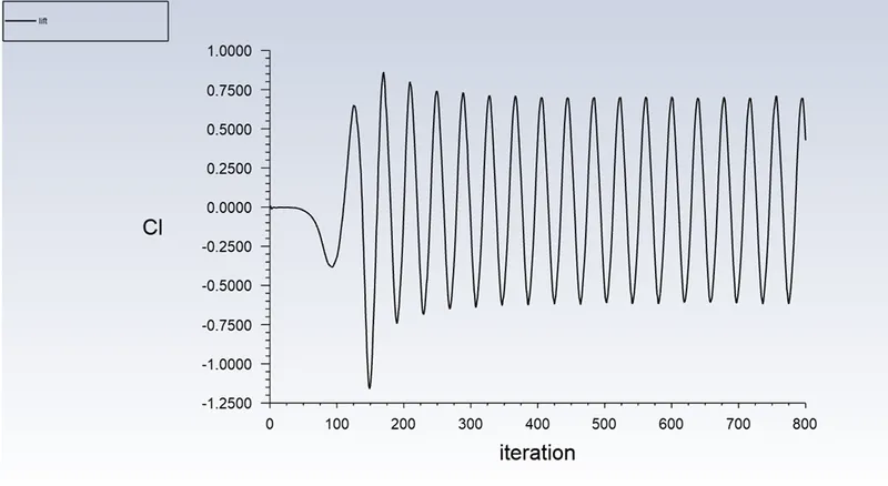
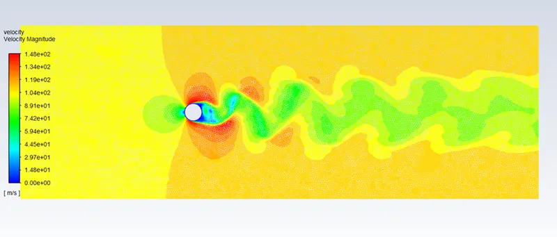
So, we can see that after 250 iterations in vertex medium it starts converging and also after 300 iterations our lift coefficient also start converging, so the convergence is approx. 300 and the lift, drag coefficient are given below the contour of velocity:

Cd=1.1730212 (1.7489542693% error)

Cl=0.42626866

CASE 4, when we have REYNOLDS NO. 10000: so, for re 1000, I ran it for 800 iterations and the residual plot is stabilizing after 300 iterations and also other plots are shown below

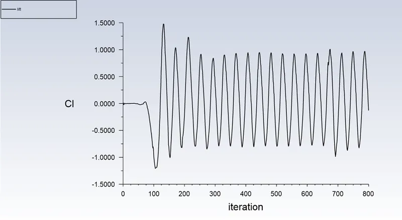
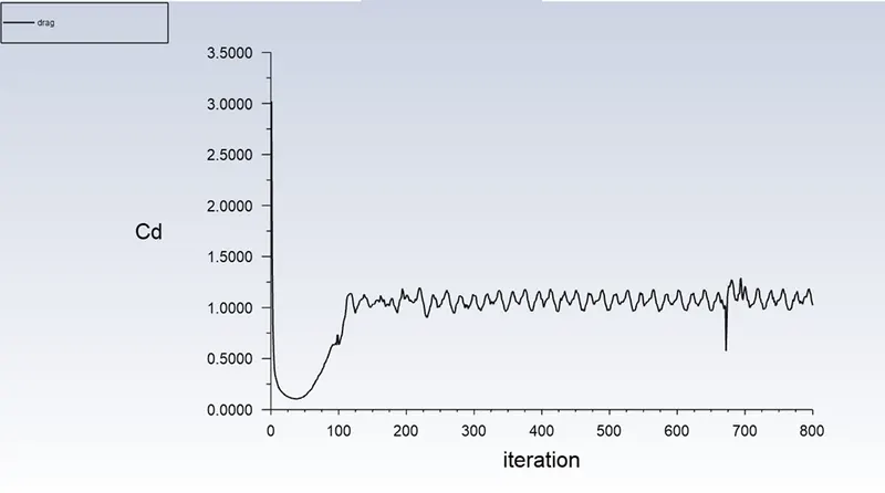
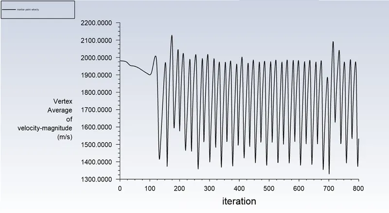
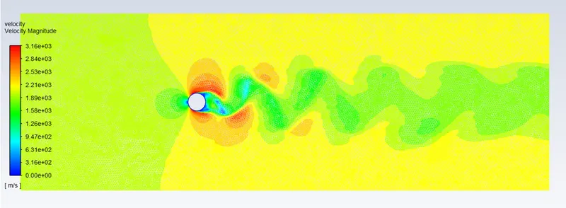
So, from the above plot we can see that after 275 iterations the plot of vertex medium and lift coefficient start converging and the value for both lift and drag coefficient along with velocity contour is given below:

Cd=1.0230364 (0.5419541498% error)

Cl= -0.12945129

CASE 5, when we have REYNOLDS NO. 100000: in this case we will get our required value of drag coefficient but the vertex medium, drag and lift coefficient are fluctuating it means at higher Reynolds no. there is a lot fluctuations and no convergence except for residuals it shows the same pattern after 400 iterations we can’t say that it is convergent but though it is stable if I ran it fir more then 4500 iterations an unknown (to me) effect starts also there is no convergence for any plots I ran the fluent for 1300 iterations to get my minimum error value, the plots , contours and the value for lift, drag coefficient are given below:

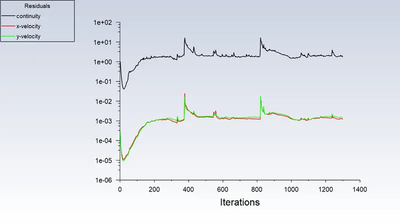
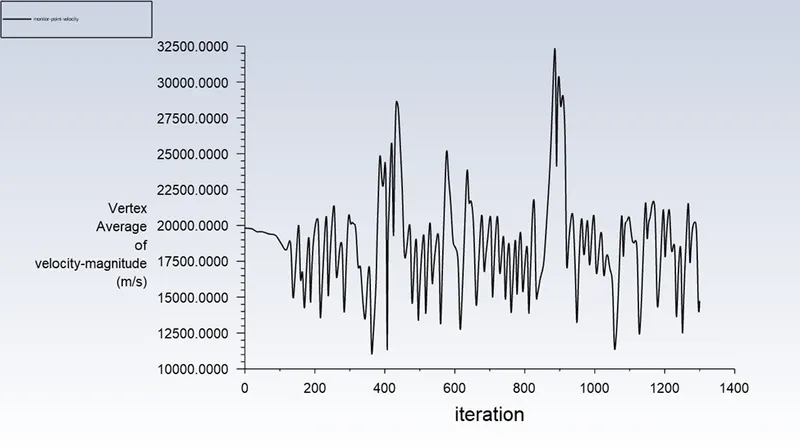
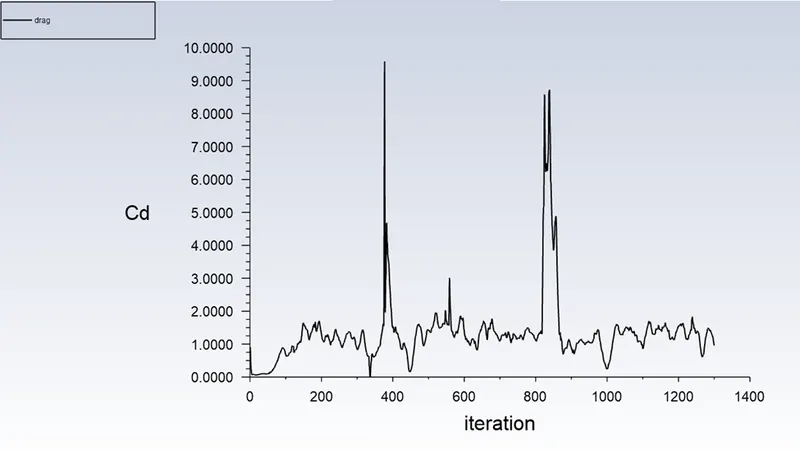
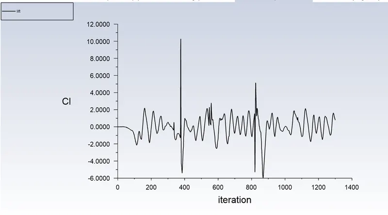
The value of Cd and cl along with velocity contour are given below:

Cd=0.95867492 (0.5245954584% error)

Cl=0.7802746

Now from above all the cases,

Cases	Cd	Cl	Percentage error of drag coefficient
Case 1, Re 10	3.3397778	-0.0003237437	0.462973339%
Case 2, Re 100	1.3593551	0.12143854	0.8797099223%
Case 3, Re 1000	1.1730212	0.42626866	1.7489542693%
Case 4, Re 10000	1.0230364	-0.12945129	0.5419541498%
Case 5, Re 100000	0.95867492	0.78027492	0.5245954584%

CONCLUSIONS: we concluded that we are not able to calculate the strouhal no. for steady flow, as the steady modal only counts the iterations. Also, we know that strouhal no. is a frequency-based equation so for calculating the frequency, time factor is required and that is only be done in (transient modal) unsteady flow.

Also, we concluded that as the Reynolds no. increase the drag coefficient starts decreasing as we see that after every increase in Reynolds no. there is decrease in drag coefficients but in case 5 of part 2, we can able to see that things get slightly change there is increase in drag and decrease in lift

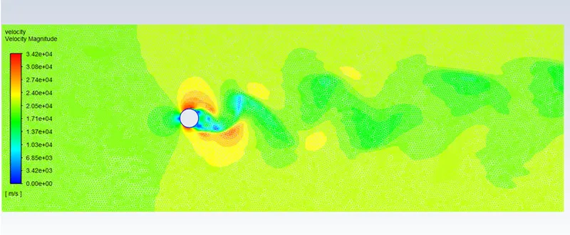
For re 10 no vortex shedding street is seen. As we increase the re from 100 to 1000, we can able to see effective vortex shedding, but for re 10000 the vortex shading is less in comparison to re 100 and re 1000 and street formation is very prominent and for re 100000 vertex street with very small height can be seen

Higher the Reynolds no. more we get the difficulty to get the convergence like in the 5^th case of part 2 we have a fluctuation that can not be able to converge whether you run the fluent for above 4000 iterations you will not get any type of required convergence for any plot in this case.

REFERENCES:

https://en.wikipedia.org/wiki/Drag_equation

https://www.grc.nasa.gov/www/k-12/airplane/dragco

https://sciencedemonstrations.fas.harvard.edu/presentations/vortex-shedding

https://www.researchgate.net

not able to upload ansys archieve file because of the size