Week 4 - CHT Analysis on Exhaust port
CHT Analysis on Exhaust port
Objectives:
Give a brief description of why and where a CHT analysis is used.
Conjugate heat transfer (CHT):
The Conjugate Heat Transfer (CHT) analysis type allows for the simulation of heat transfer between solid and fluid domains by exchanging thermal energy at the interfaces between them. Typical applications of this analysis type exist as, but are not limited to, the simulation of heat exchangers, cooling of electronic equipment, and general-purpose cooling and heating systems.
The contemporary conjugate convective heat transfer model was developed after computers came into wide use in order to substitute the empirical relation of proportionality of heat flux to temperature difference with heat transfer coefficient which was the only tool in theoretical heat convection since the times of Newton. This model, based on a strictly mathematically stated problem, describes the heat transfer between a body and a fluid flowing over or inside it as a result of the interaction of two objects. The physical processes and solutions of the governing equations are considered separately for each object in two subdomains. Matching conditions for these solutions at the interface provide the distributions of temperature and heat flux along the body-flow interface, eliminating the need for a heat transfer coefficient.
Why CHT analysis is used:
Computational Fluid Dynamics (CFD) and more specifically conjugate heat transfer (CHT) analysis can accurately predict heat transfer by simultaneously solving all the relevant solid and flow field heat transfer processes for example, conduction through solids, free and forced convection in the gases/fluids and thermal radiation
The CHT approach has an advantage over FE thermal analyses in that wall heat transfer coefficients and their local variations on surfaces are directly calculated within the model rather than based on simplified empirical calculations. The CHT approach, therefore, has benefits for those applications where heat transfer is either non uniform or difficult to calculate empirically.
Where is CHT analysis used:
Starting from simple examples in the 1960s, the conjugate heat transfer methods have become a more powerful tool for modeling and investigating natural phenomena and engineering systems in different areas ranging from aerospace and nuclear reactors to thermal goods treatment and food processing from complex procedures in medicine to atmosphere/ocean thermal interaction in meteorology, and from relatively simple units to multistage nonlinear processes.
Heat transfer co-efficient:
The heat transfer coefficient or film coefficient, or film effectiveness, in thermodynamics and in mechanics is the proportionality constant between the heat flux and the thermodynamic driving force for the flow of heat (le, the temperature difference, A7):
The overall heat transfer rate for combined modes is usually expressed in terms of an overall conductance or heat transfer coefficient, U. In that case, the heat transfer rate is:
Q=hA(T₂-T₁)
where
A: the surface area where the heat transfer takes place, m²
To temperature of the surrounding fluid, K
T₁: temperature of the solid surface, K
The general definition of the heat transfer coefficient is:
h= q/delta t
CHT Analysis on Exhaust port silumation
For base mesh
Step 1 :
setup geomerty
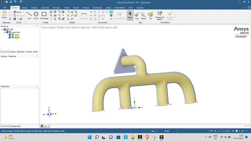
Use volume extract method make a new component as solid and fulid
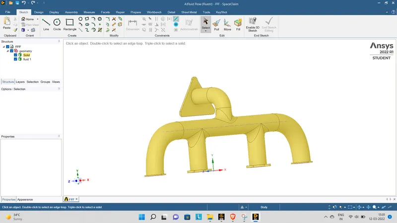
Make sure to check the share topology and shareper option to geometry to share
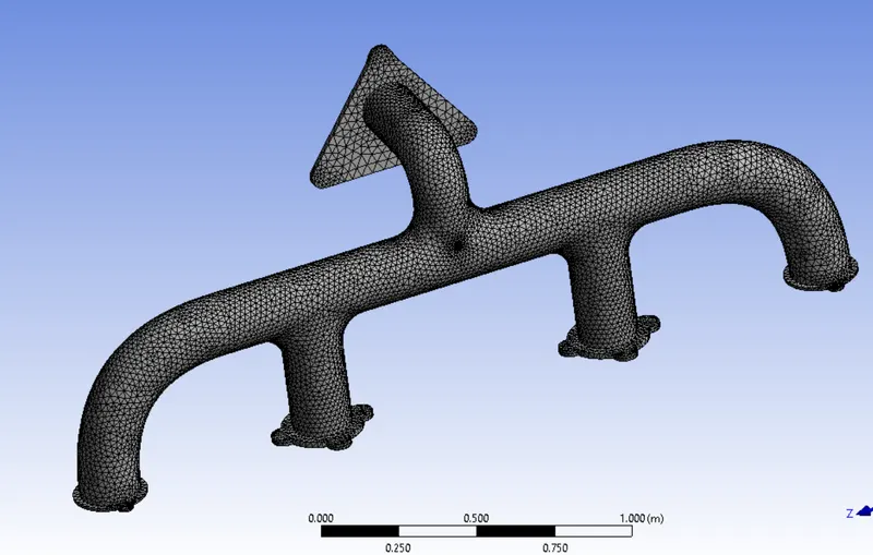
Case 1 base mesh simulation

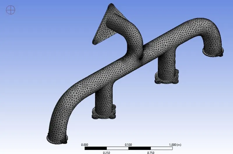
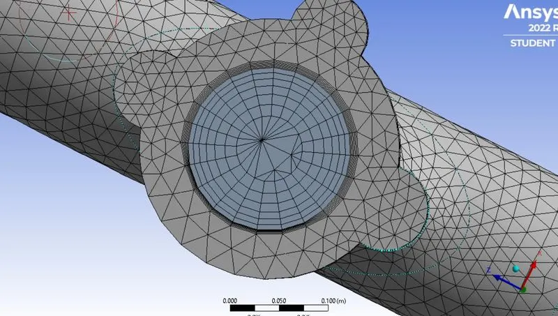
use 0.1m base mesh
0.05m as inflation layer
0.05 outer sizing wall
elenments 2
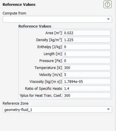
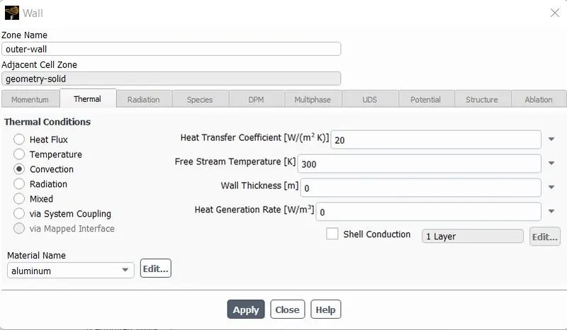
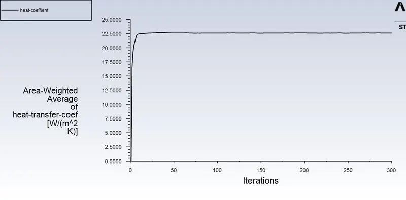
iniltilize ans run up tp 300 iterations
Results
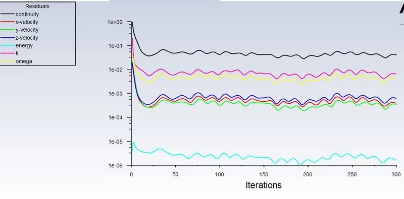
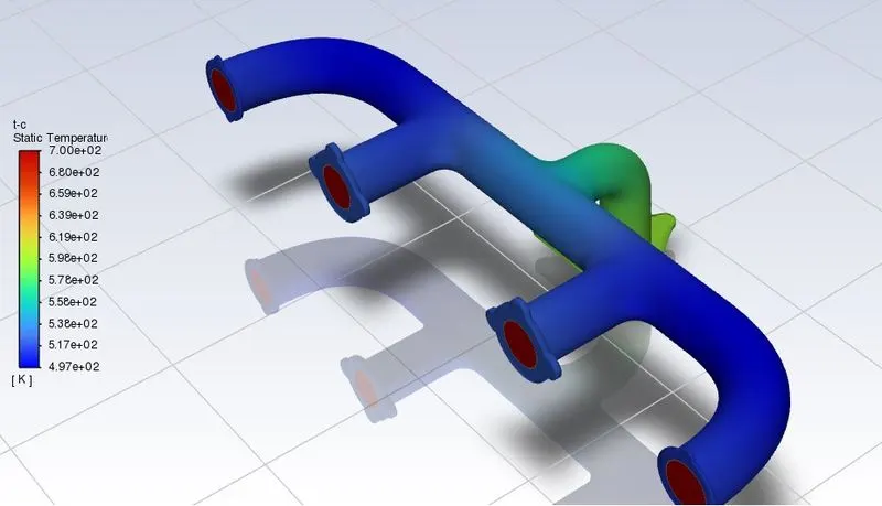
case 2 refined meshing
Step 1 : creating geometry same as base mesh process
Step 2 : Meshing
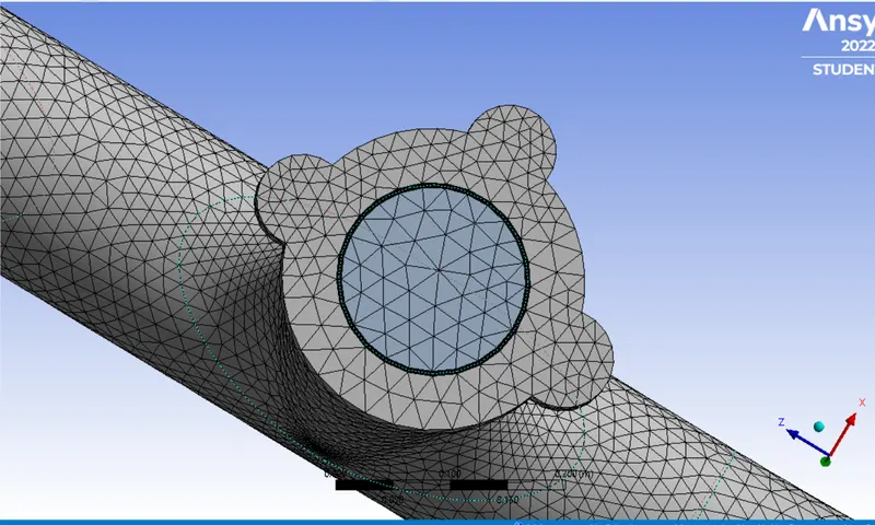
Inflation layer is calculated by the Y+ valve . we used first layer method
Hence we are using turbulance module as K omega we taken Y9 value as 3
according to the calculation we got thikness as 2.2e-4 m .
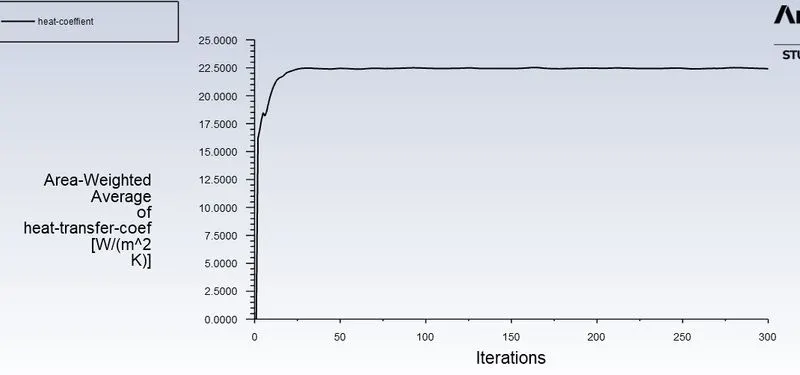
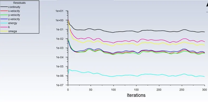
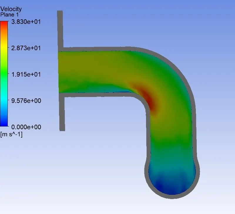
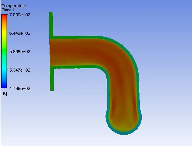
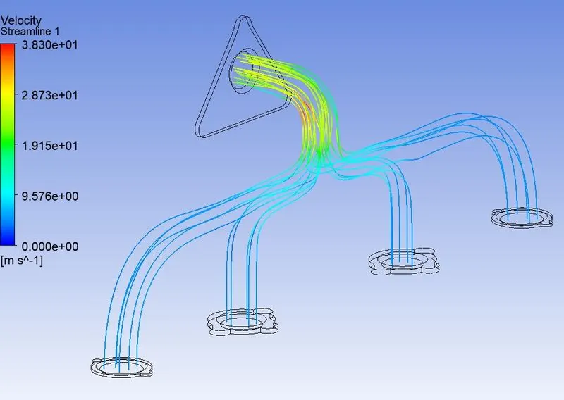
For refind mesh elenments are 4,500,000
HEAT TRANSFER COEFFICIENT VERIFICATION.
Heat Transfer coefficient at boundary surface is often calculated using Nusselt number. Hence to verify the HTC obtained from the CHT analysis we first need to calculate the theoretical value of the Nusselt number.
For a turbulent flow inside a smooth pipe, Nu number is given by Dittus-Boelter equation.
(Nu) 0.023 (Re) (Pr) 1
Also,
Nu AL k 2
D = Diameter of the circular duct,
Pr = Prandtl number,
n=0.4 for the fluid being heated, and n = 0.3 for the fluid being cooled.
Nu = Nusselt Number
Re Renolds number
Hence, using the value of Nu from (1) we can find the value of the heat transfer coefficient, h from equation (2) and verify it with the actual results obtained from the above simulations.
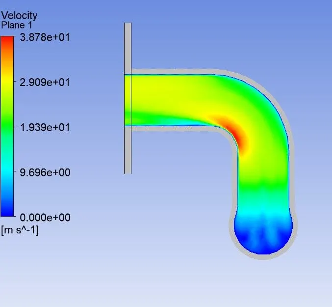
By examining the velocity contours at the plane we can understand that there is a high velocity at the bent which implies a high Reynold number From the above relation, we can say that as Re increases Nu increases as well, which in turn increases the heat transfer coefficient.
Factors affecting the accuracy of prediction from simulations are
• Inflation layer - It increases the quality of mesh near the boundary interface and it can capture smooth plots of heat transfer coefficient.
• Grid size and shape -The grid size as it decreases the quality of the mesh will increase and also the shape of the mesh also matters and gives more accurate result.
• Setting share topology Mesh should be conformal for smooth transferring of mesh in different zones
Conclusions:
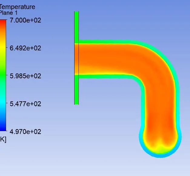
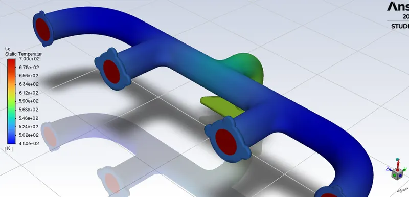
In temperature contour, even our inlet temperature of the air is 700k (for fluid), it doesn't get the transfer to the outer solid body as the temp. remains the lowest and as we go towards the outlet, we see a gradual increase in temperature. As we increased the mesh size, the solid region maximum and minimum temperature also increase.
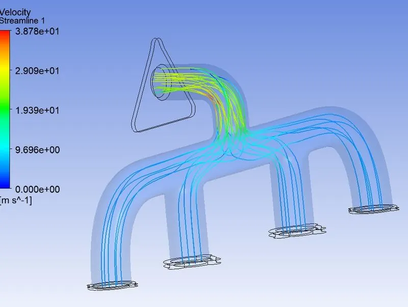
For Streamline velocity plot, the velocity at the inlet is zero and as we move towards the outlet we see a gradual increase in velocity and maximum at the curvature of the throat. This happens because of total mass conservation, as there are 4 inlets and a single outlet
Here, velocity is directly proportional to temperature, and hence the maximum temperature is also produced at the curvature of the throat on the plane where the maximum heat gets transferred from the fluid region to Solid zone. Therefore, the highest Wall heat transfer Coefficient is obtained at that location.
For Wall Heat Temperature Coefficient, it raises from102.5 W/m^2-k to 210.7 W/m^2-k as the mesh number of elements increase and moshes size decrease.
As the no. of elements increases the Velocity, Temperature and Wall Heat Transfer Coefficient increases.