Week 4 - CHT Analysis on Exhaust port

Introduction:

Exhaust port:

The exhaust manifold is a key component of 4 stroke I.C. engine. the exhaust manifold is mounted on the cylinder head of the engine. the exhaust manifold collects the exhaust gases from multiple cylinders into one pipe. at the exhaust stroke, the exhaust valve opens and the inlet valve remains closed that time piston starts moving from the bottom dead centre to the top dead centre sweep out burnt gases from the cylinder. these exhaust gases sweep out from the cylinder and transfer through a catalytic converter.

the temperature of these exhaust gases are about 800 degrees Celcius and the pressure range is 100-500 kpa. this temperature and pressure are experienced during the exhaust stroke. the exhaust manifold is made up of grey cast iron is a type of cast iron that has a graphite microstructure because of its ability to tolerate fast and severe temperature changes.

Why CHT analysis is used?

When the engine works hard the exhaust manifold can run with red hot. so we have to investigate the complete behaviour of the exhaust manifold. only flow or only thermal analysis is not sufficient for engine exhaust system but we have to understand the thermal behaviour of structure due to fluid parameters or vice versa by coupling called conjugate heat transfer.

In certain critical applications where working temperature is very high, it is necessary to calculate the temperature distribution in the solid to ensure that it should not cross the metallurgical limit. The Selection of the material and wall thickness is largely dependent on the wall temperature distribution in the solid. Hence, it is necessary to solve the energy equation of the solid along with the fluid flow equations, commonly known as the conjugate heat transfer problem.

This type of problem differs from commonly encountered heat conduction problems, as the temperature of the fluid which is used to cool (or heat) the solid is not known a priori. Instead, the fluid temperature is calculated at the same time as the solid temperature.

Where CHT analysis is used?

CHT is used to describe the processes that involve the energy exchange between solid and fluid domains due to interaction between them and is frequently encountered in a variety of engineering applications such as internal combustion engines, turbomachinery, heat exchangers etc.

What is CHT?

For conjugate heat transfer analysis, solid material conduction and fluid convection are analysed simultaneously. the conductive heat transfer in the solid region is coupled to convective heat transfer in neighbouring fluid flow.

I Baseline simulation:

There are five steps to simulate CHT analysis of the exhaust port.

1. Geometry

2. Mesh

3. Setup

4. Solution

5. Result

1. Geometry:

first, we import geometry file in space claim. then after detect and remove the extra edges that are not needed to define the shape of the model.

go to "Prepare". then click on the "extra edge" and select the edges in the geometry. then click on " green colour right tick"

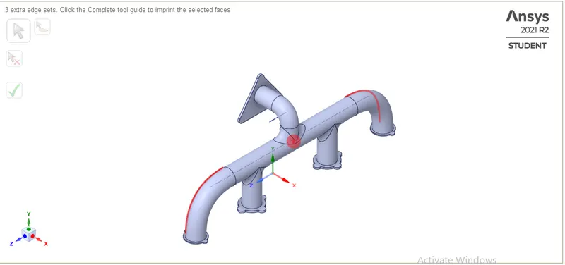
Figure 1.1: extra edges selected

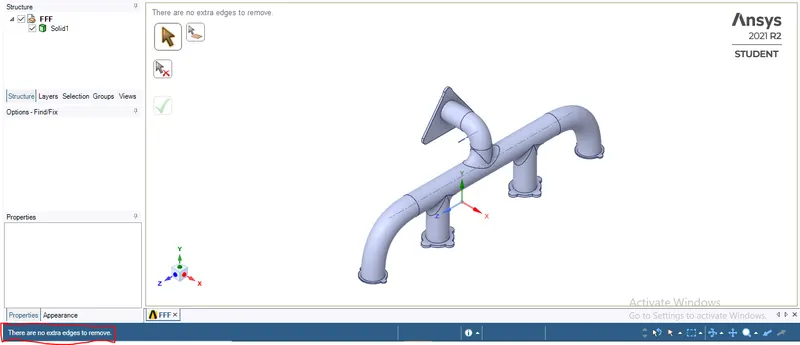
Figure 1.2: extra edges have been removed

now we extract the fluid volume from the model by clicking on the "prepare" tool. then click on "volume extract" then click on "select edges". Click on " green tick"

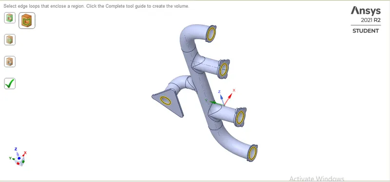
Figure1.3: selected edges to remove fluid volume

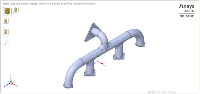
Figure 1.4: Fluid volume has been created

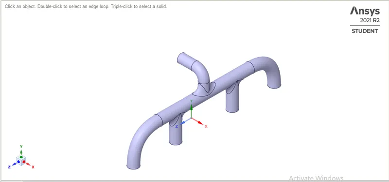
Figure 1.5: Fluid part of the model

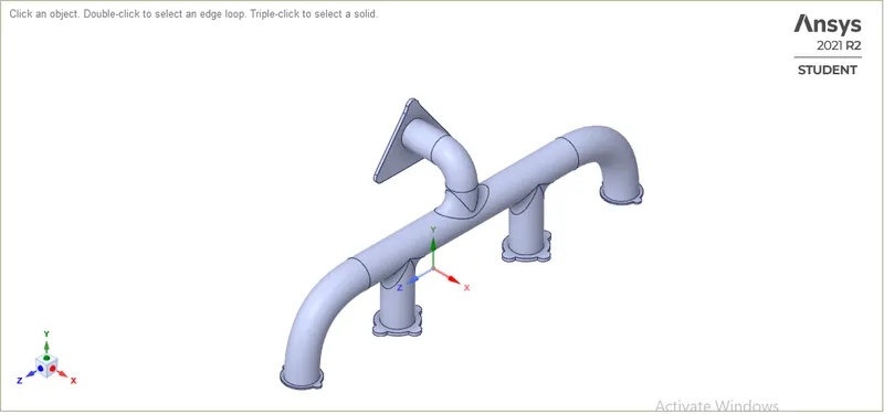
Figure1.6: Solid part of the model

Here step 1 of geometry has been completed. it is ready to do mesh.

2. Mesh:

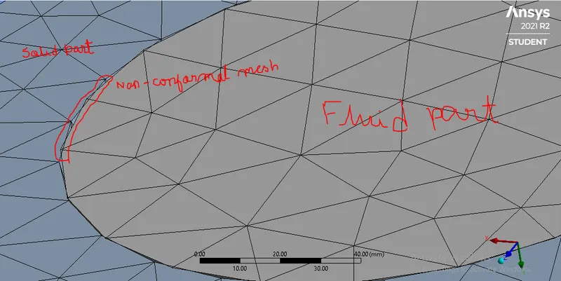
Figure 2.1: Non-conformal mesh (nodes are not shared at the interface)

To make the conformal mesh, use share topology.

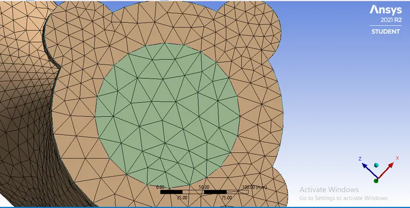
Figure 2.2: Conformal mesh (nodes are shared at the interface)

now create a Named selection

• inlets
• outlet
• outer wall convection

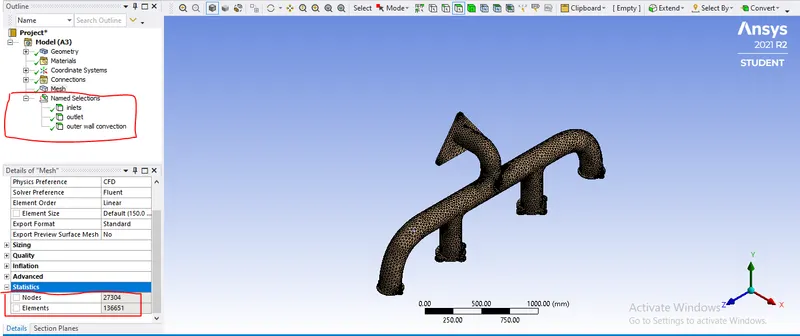
Figure 2.3: named selection and baseline mesh

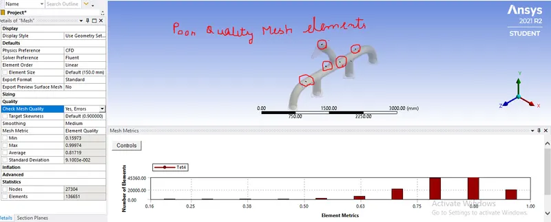
Figure 2.4: Mesh quality

in the above figure 2.3, the number of elements is 136651. we can increase the mesh elements more by further refinement to improve mesh quality. since we have a mesh limit of 512000 for the student version. so let's do further refinement.

3. Setup:

used following things

• Pressure based solver
• steady time
• Turn on " Energy"
• k-epsilon(2 eq) model

Material:

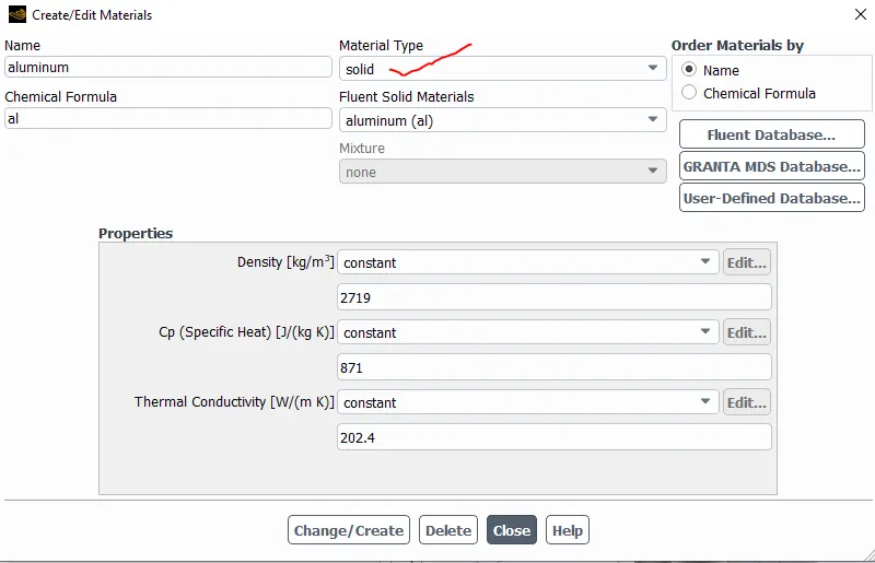
Figure 3.1: Material properties

Boundary conditions:

• inlet velocity=5 m/s
• inlet temperature=700K
• outer wall convection heat transfer coefficient, h=20 w/m2K

4. Solution:

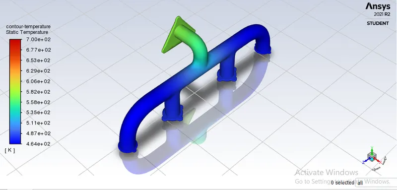
Figure 4.1: Static temperature

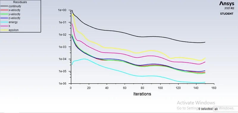
Figure 4.2: Residuals of continuity, momentum and energy equation

5. Result

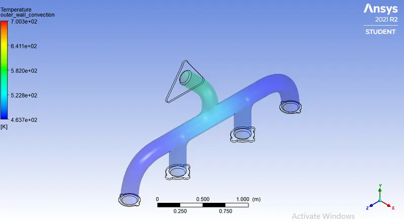
Figure 5.1: Temperature distribution at the outer wall

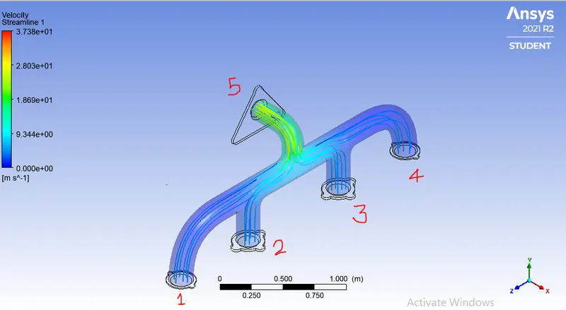
Figure 5.2: velocity streamline

Apply mass conservation equation, the total flow rate at inlets=flow rate at the outlet

`Q_1+Q_2+Q_3+Q_4=Q_5`

`A_1V_1+A_2V_2+A_3V_3+A_4V_4=A_5V_5`

here cross-section area of each inlet and outlet are the same. `V_1+V_2+V_3+V_4=V_5`

Hence at outlet velocity will be more than the inlet. therefore Reynold's number, Re at the outlet will be more because Re is directly proportional to velocity. and flow will be turbulent.

as we know for turbulent pipe flow, `Nu=(hD)/K=0.023 Re^0.8 Pr^n`

Hence there will be a more convective heat transfer coefficient because, from the above correlation, the Convective heat transfer coefficient is directly proportional to Re.

Convective heat transfer from the fluid to solid is `Q=hADelta T`. therefore solid part at the outlet has more temperature as we can see in figure 5.3.

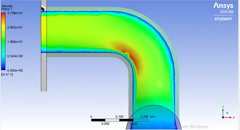
Figure 5.3: Velocity contour in XY plane

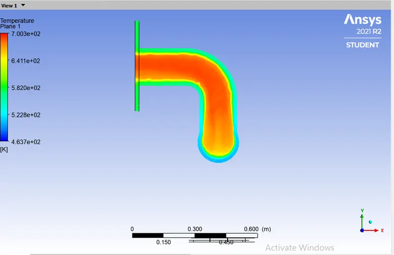
Figure 5.4: Temperature contour in XY plane

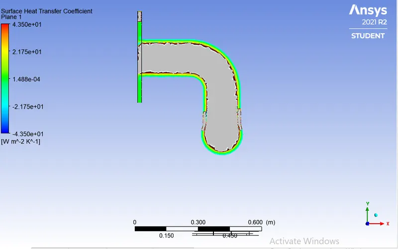
Figure 5.5: Surface heat transfer coefficient

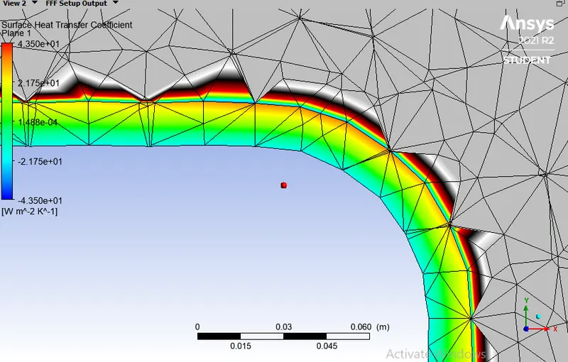
Figure 5.6: Zoom view of Surface heat transfer coefficient

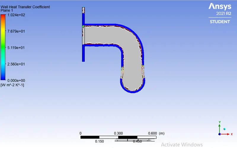
Figure 5.7: Wall heat transfer coefficient

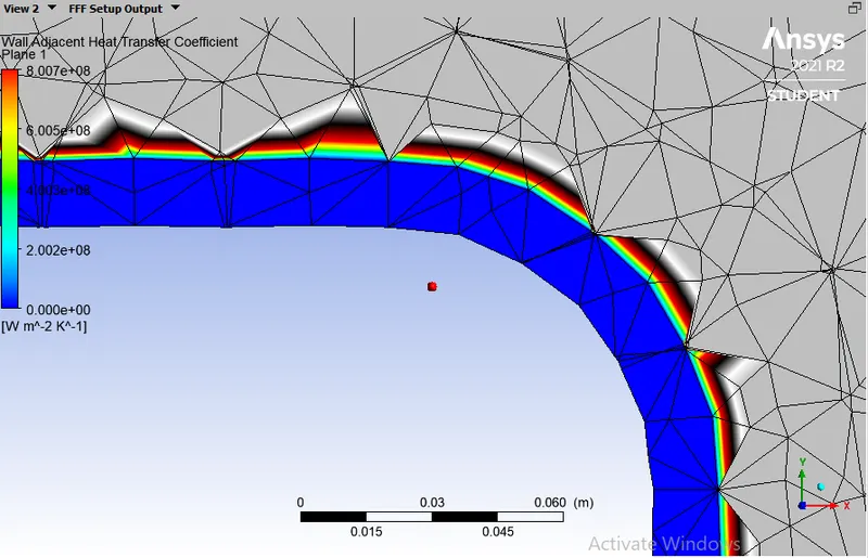
Figure 5.7: Zoom view of Wall heat transfer coefficient

Case II: Refinement

2. Mesh:

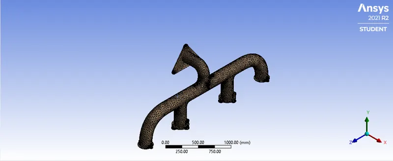
Figure 2.1: complete model contains both solid and fluid parts.

Now we hide the solid part of the model.

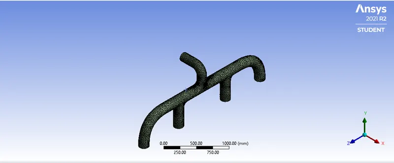
Figure 2.2: Solid part hidden. only fluid part is visible.

now create an Inflation layer in the Named Selection tree

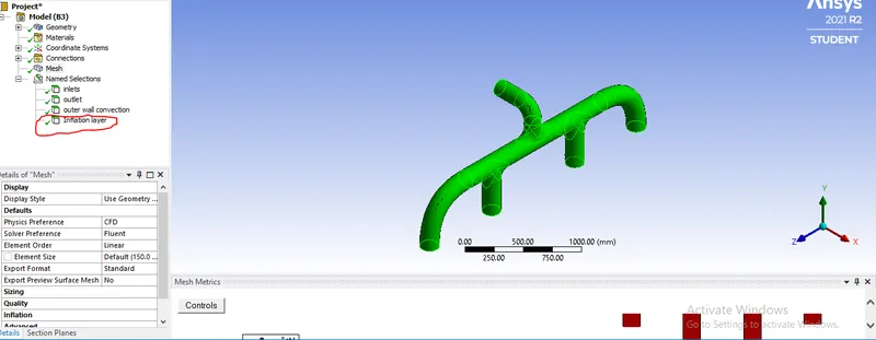
Figure2.3: inflation layer in Named selection tree.

Figure 2.4: inflation layer details

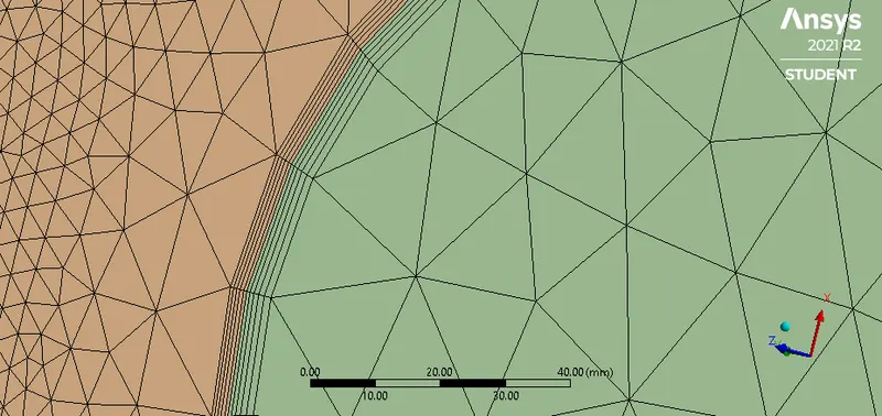
Figure 2.5: Created inflation layer

now we decrease the body size (element size) to 7 mm

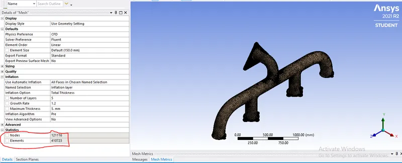
Figure 2.6: Refined mesh

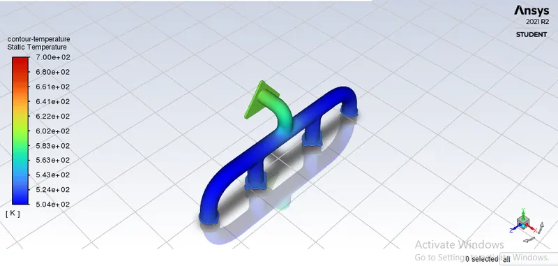
Figure: contour of static temperature

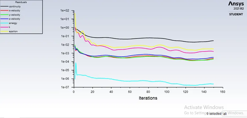
Figure: Residual plot

5. Result:

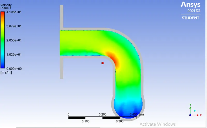
Figure 5.1: Velocity contour in XY plane

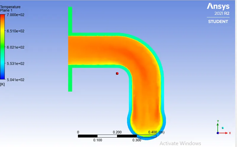
Figure 5.2: Temperature contour in XY plane

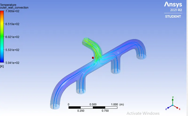
Figure 5.3: Temperature streamline

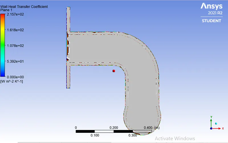
Figure 5.4: Wall heat transfer coefficient

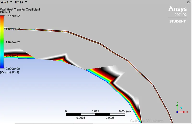
Figure 5.5: Zoomed section of Wall heat transfer coefficient

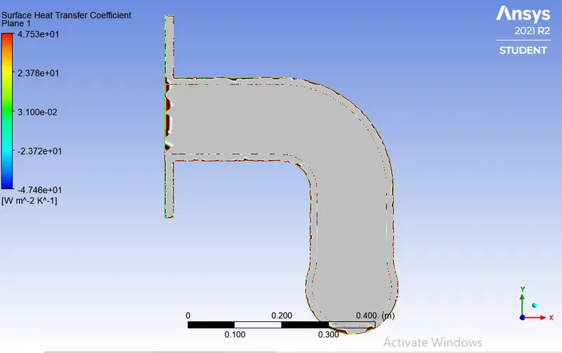
Figure 5.6: Surface heat transfer coefficient

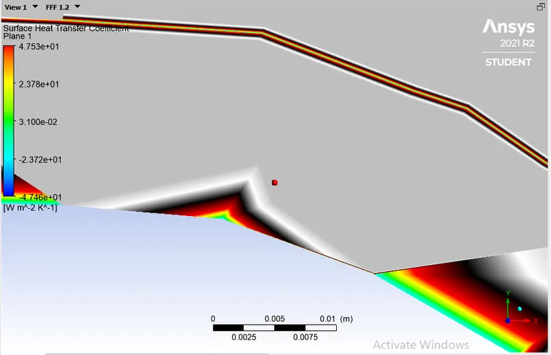
Figure 5.7: Zoomed view of surface heat transfer coefficient

How would you verify if the HTC predictions from the simulations are right? On what factors does the accuracy of the prediction depend on?

as we know for turbulent pipe flow, `Nu=(hD)/K=0.023 Re^0.8 Pr^n`

by using the above correlation, we find convective heat transfer coefficient(h) analytically. and compare it with convective heat transfer coefficient(h)numerically what we got in above figure. this is the way to verify the HTC.

Conclusion:

• flow and thermal analysis gives acuurate result based on desired Y+ value.
• simulation with refinement at the interface of solid and fluid part gives proper heat transfer at their interface.