CHT Analysis on Exhaust port using Ansys Fluent.

The description of CHT analysis and its applications:

The term conjugate heat transfer can be used to describe the processes which involve a temperature variation within the solids and fluids themselves due to the thermal interaction between the solid and the fluid.

During CHT the heat transfer can take place from solid media to the fluid media and vice-versa. This is because fluids flow around solids or between solid walls, and also the solids are mostly immersed in a fluid.CHT analysis is beneficial in engineering applications because it shows the heat exchanging capabilities between the two surfaces in the engineering device and various optimization can be done to improve the thermal characteristics of the devices.

Thus, this can be used to improve the heat transfer rate wherever required. It also helps us to identify the key parameters that enhance the fluid flow and heat transfer within the system. Conjugate heat transfer corresponds with the combination of heat transfer in solid and fluid. In solids, conduction often dominates, whereas, in fluids, convection dominates. Efficiently combining heat transfer in fluids and solids is the key to designing effective coolers, heaters, or heat exchangers. Forced convection is the most common way to achieve a high heat transfer rate. In some other applications, the performance is further improved by combining convection with phase change.CHT can be performed to improve the cooling performance of water jackets and increase engine life.

ADVANTAGES

1. The Conjugate Heat Transfer setup replaces the empirical relation of proportionality of heat flux to temperature difference with heat transfer coefficient. The wall heat transfer coefficients & their local variations are directly computed within the model and do not involve the solving of complex empirical relations. Thus the simulations are carried out much faster.

2. As long as the boundary conditions are accurately defined, the solutions are highly accurate due to the simplicity of the CHT model.

3. There is no limit for the number of surfaces and hence can be applied for a large number of regions in a given assembly.

4. Since the CHT model is a combination of the heat transfers in both a solid & fluid model, it can be applied for all combinations of interactions (i.e. Solid - Fluid interaction, Solid - Solid interaction and Fluid - Fluid interaction).

APPLICATIONS

The CHT method is a powerful tool for simulating & analyzing flows in a variety of different applications such as designing different vehicles, machines and also investigating natural phenomena such as thermal interactions in the atmosphere.

VERIFICATION OF SIMULATION

In this numerical analysis, we have carried out the verification of the solution obtained from the simulation with the analytical result in which we used the k-`epsilon` equation to capture the flow.

Analytical solution

There are three different situations through which heat exchange takes place in the given exhaust manifold model. The first scenario begins with heat being conveyed from the exhaust gas to the pipe walls through forced convection during fluid flow from the inlets of the manifold to the exhaust outlet. The convected heat then travels from the internal surface of the manifold to the external surface by conduction through the solid pipe wall which is then convected the to surrounding, in this case, by natural convection as it is assumed that both the model and the air surrounding it are in a stationary condition. In this numerical study. The variable of interest is the wall heat transfer coefficient on the internal surface of the pipe. Therefore, based on the boundary condition available with regards to the given model the heat transfer properties will be evaluated.

Forced convection- Exchange of heat from exhaust gases to the pipe internal surface.

As the Reynolds number calculated for the flow suggests that the flow behavior is turbulent in nature. The Dittus-Boelter heat transfer coefficient correlation can be used to calculate the Nusselt number which is the ratio of convective heat transfer to conductive heat transfer.

`Nu =0.023. Re^(5/4).D.Pr^(n)`

where

D=Inlet pipe diameter

Pr=Prandtl number=`mu.Cp/k`

`mu`=Dynamic viscosity.

`Cp`=Specific heat of the fluid.

`k`=Thermal conductivity of the fluid.

`n`=0.3

The above equation is also valid for the given boundary condition based on the limitations defined below

`0.6<=Pr=0.744<=160`

`ReD=58189.896>10,000`

`(L/D)>10`

We know that the Nusselt number is Mathematically written as `Nu=h/(k/l)`

where L = characteristic length k = thermal conductivity h = convective heat transfer coefficient.

Solving for h we get heat transfer coefficient as 19.428 `W(m^2.K)` using thermal conductivity of air as 0.0242 `W/(mK)` it should be noted that the Dittus-bolter heat transfer coefficient correlation was observed to be accurate in the range of ±15% and works best when the pipe surface is very smooth duct.

R = (Convection resistance) Out + Wall Conductivity resistance+ (Convection Resistance);

R=

hout

`R=(1/hout)+(L/K)+(1/(h.epsilon))`

`R=(1/20)+(0.015/202)+(1/(h.epsilon))`

Here, at node point: q = 6987.5 `W/(m^2K)`, Bulk Temperature = 682.31 K

Therefore,

After substitution we get,

AT 682.31-300 = 381.31 K

hi= 215.55 `W/m^2K`

PROCEDURE OF SIMULATION

Geometry

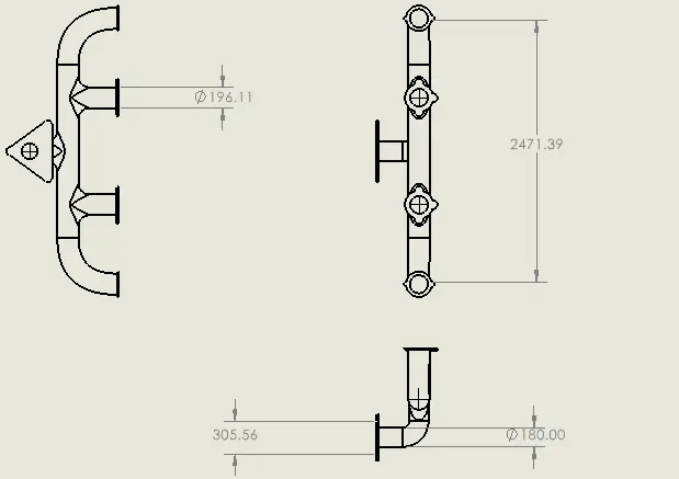
Fig 1: Dimensions of Exhaust port

1) Import the geometry in Spaceclaim.

2) Use geometry clean-up tools if having any problems in geometry such as extra edges.

3) Extract the fluid volume (This operation is only successful if our geometry doesn't have any problem .)

4) Share the topology in design.

5) Make solid and fluid volume as a new component. (RC`rarr`FFF`rarr`create a new component).

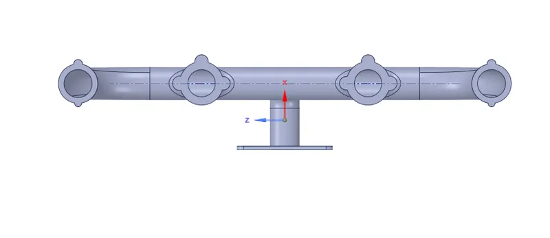
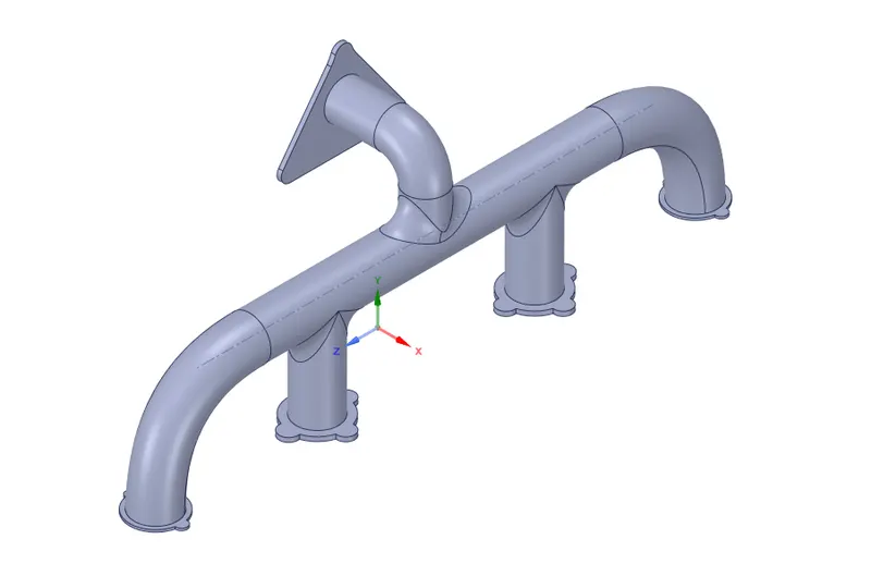
Fig 2: Exhaust Manifold Geometry

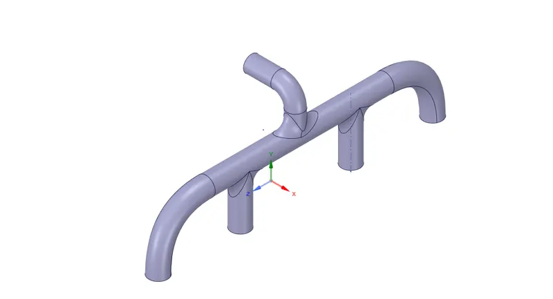
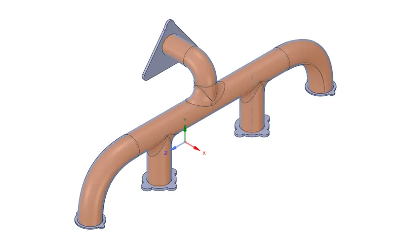
Fig 3: Fluid Volume Enclosed by Geometry

Meshing

1) Create named selection as inlets(select all four faces), outlet and outer-wall-convection(double click to select all outer faces).

2) For baseline mesh we will use the patch-conforming method with a 100mm mesh size.

3) After using baseline mesh we will refine the mesh with inflation layers for a suitable turbulence model by automatic inflation using named selection and reducing mesh size to 15mm.

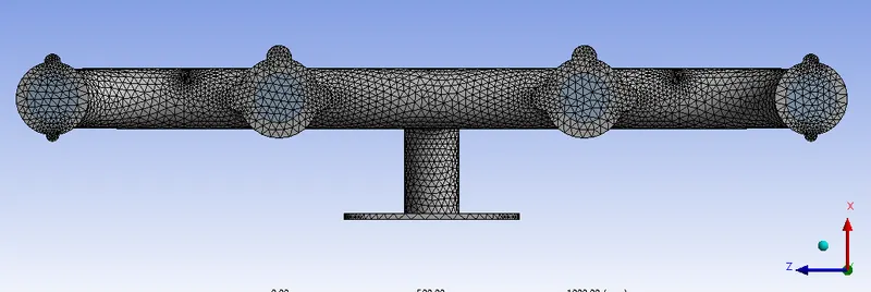
Fig 4: Baseline mesh

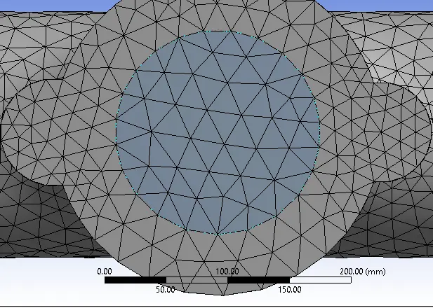
Fig 5: Conformal Mesh

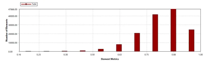
Fig 6: Mesh Metrics

Fig 7: Inflation for k-`omega` model with first cell height as 0.05mm

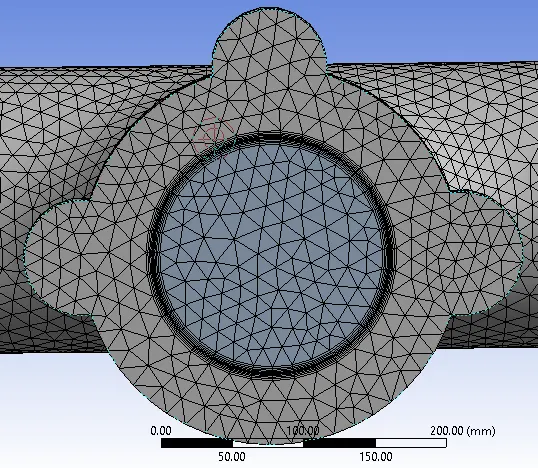
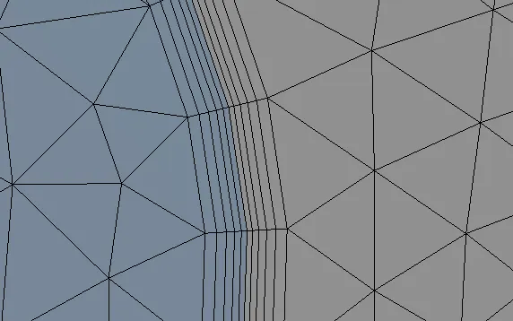
Fig 8: Inflation layer with total thickness as 5mm for k-epsilon model.

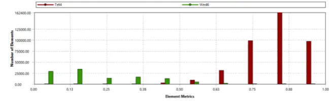
Fig 9: Mesh Metrics with inflation

Solver Setup:

1) Type: Pressure Based(Mach No.<0.3), Steady simulation.

2) Energy Equations should be turned on to take the heat transfer effect into account.

3) Turbulence models: k-`omega` and k-`epsilon` for comparison.

4) Boundary Conditions:

a) inlet velocity= 5m/s

b) inlet temperature= 700K

c) wall convection thermal condition: convection with heat transfer coefficient=20`W/(m^2.k)` and free stream temperature=300K.

5)Material: a)Solid Volume= Aluminium

b)Fluid Volume=Air(`rho`=1.225`kg/(m^3)` and Kinematic viscosity of `1.4207x10^-5 Pa.s`

6) Initialization=Hybrid

7) Iterations=800 (whenever Solution converges iteration will stop).

CASE 1 K-`epsilon` with refined mesh

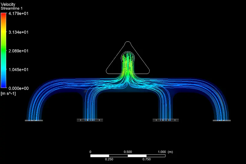
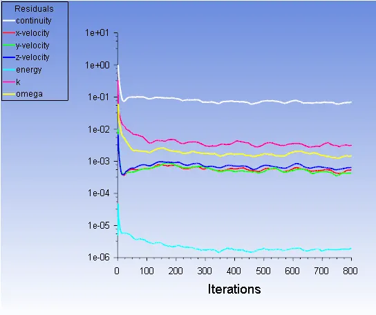
Fig 10: Streamlines Fig 11: Iterations

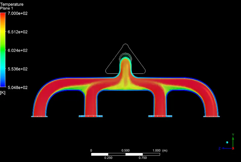
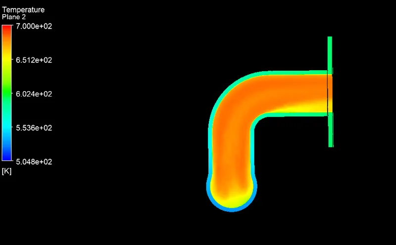
Fig 12: Temperature Distribution

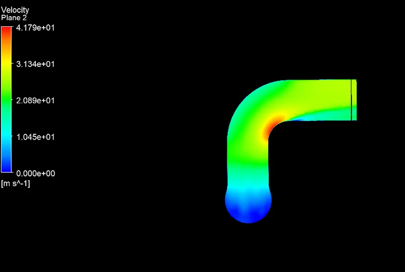
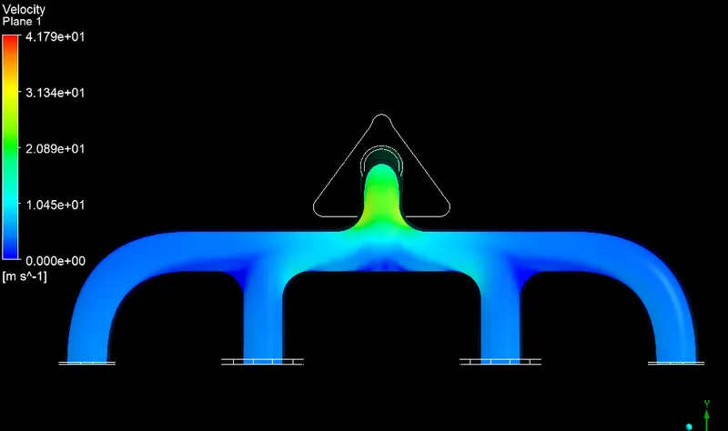
Fig 13: Velocity distribution

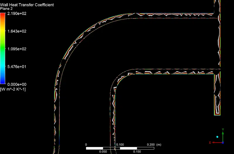
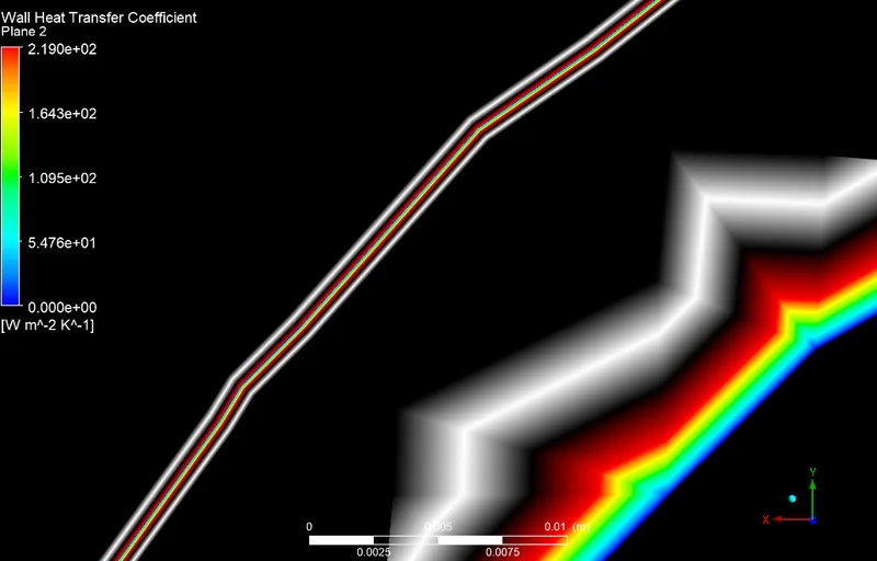
Fig 14: Wall Heat Transfer Coefficient

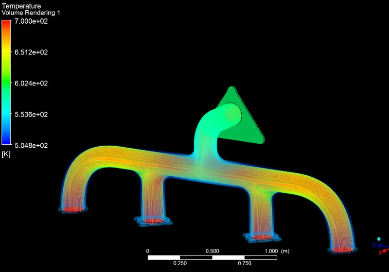
Fig 15: Volume rendering of Temperature

The solution converged at 300 iterations.

CASE 2 K-`omega` with refined mesh.

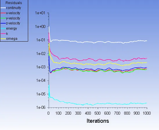
Fig 16: Residuals Plot

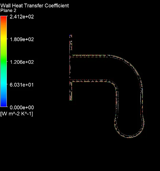
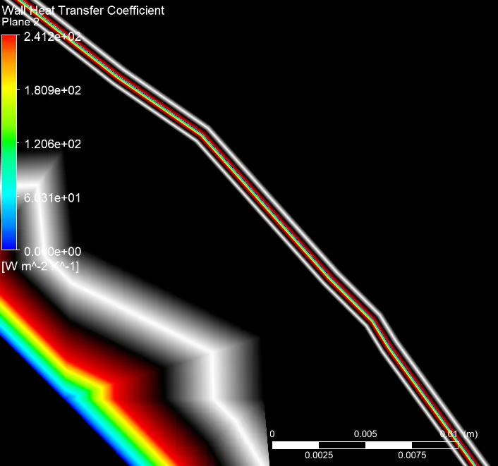
Fig 17: Heat Transfer Coefficient

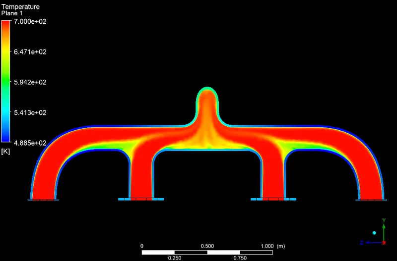
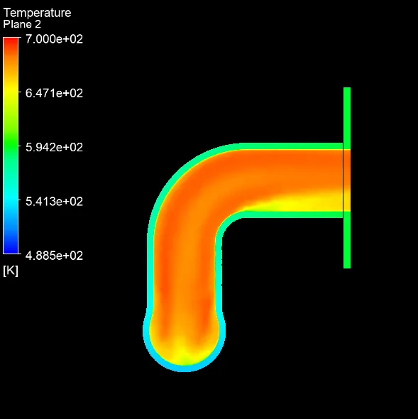
Fig 18: Temperature

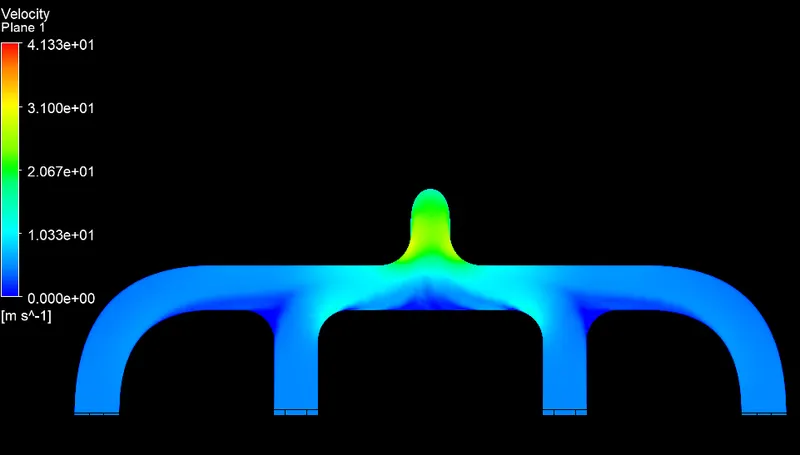
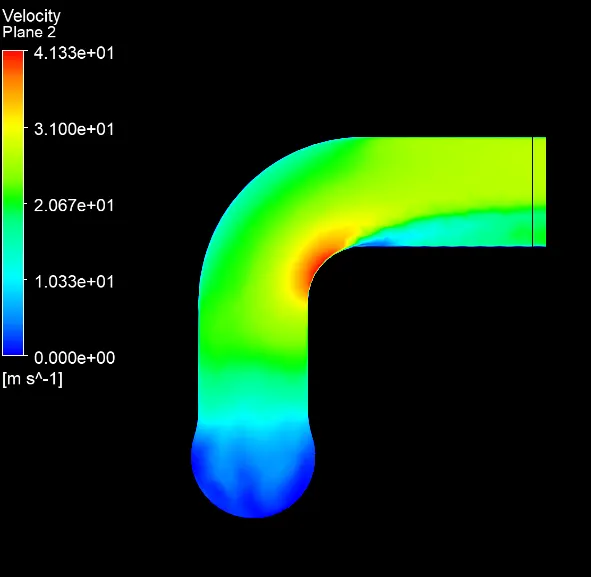
Fig 19: Velocity Contour

CASE 3 k-`omega` with baseline mesh

Iterations converged at 550.

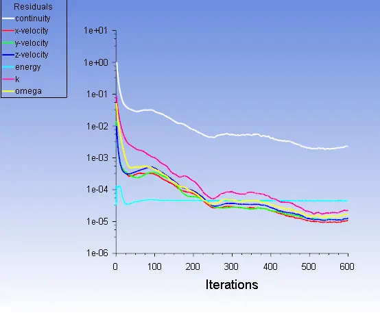
Fig 20: Residuals

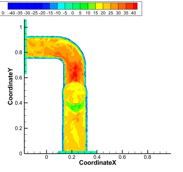
Fig 21. Surface Heat transfer Coefficient

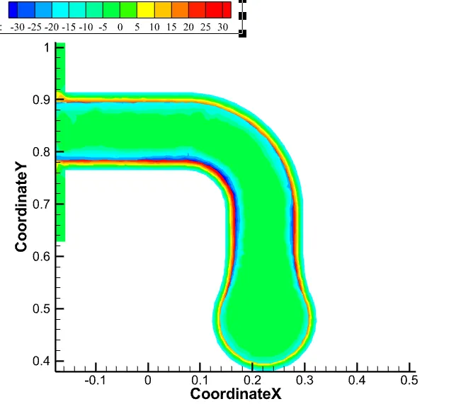
Fig 22. Surface Heat transfer Coefficient at Outlet

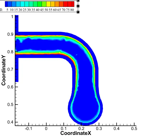
Fig 23: Wall Heat Transfer Coefficient

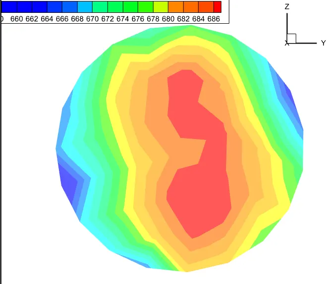
Fig 24. Outlet Temperature Contour

RESULTS

Simulation Cases	Analytical Heat transfer Coefficient (`W/(m^2.K)`	Numerical Heat Transfer Coefficient (`W/(m^2.K)	% Error
k-epsilon with baseline mesh	215.55	236.21	9.76
k-epsilon with refined mesh	215.55	219	1.6
k-`omega` with baseline mesh	215.55	241.2	11.879
k-`omega` with refined mesh	215.55	221.44	2.7325

Factors that affect the quality of prediction:

• More refined mesh leads to better results.
• Use inflation layers and apply proper Boundary conditions.
• Proper selection of turbulence model according to y+ values.

CONCLUSION

1. From the above cases output, we can say that the results are almost the same but the refined mesh gives us more smoothness and accuracy.

2. Two factors influence the performance simultaneously: (a) Flow is developing along the length and the heat transfer coefficients tend to decrease along with flow (b) Turbulence;

3. At the same time, turbulence is developing with tube rows at the bent, which would increase heat transfer coefficients.

4. The maximum heat transfer results at the bend of exit port, It is because to ensure the conservation of mass at exit port velocity should more, which results in higher velocity and increase in velocity attain a Reynolds number that is sufficient to make flow turbulent and higher Nusselt number at pipe bent at the exit, which increases Heat transfer co-efficient at that location.

5. The internal flow velocity and its characteristics are affected by the Initial velocity, Pressure, the physical features of the geometry, etc. that affect the heat transfer rates, and hence CHT analysis is essential prior to experimental analysis for better prediction life of the designed component.

6. As shown in the plots, the hot exhaust gases passing through the manifold transfer some of the heat to it via convection. The amount of heat transfer can be related directly to the velocity of the exhaust. The temperature is lower where the flow is stagnating or is moving at the inlet velocity. As the velocity increases, so does the Reynolds number and hence the amount of heat transferred.

7. Best method to predict the accuracy of the result is by comparing the nusselt numbers from experiments and numerical results. The other method to verify is by comparing the results from published experimental results.