Week 4 - CHT Analysis on Exhaust port

AIM – Steady state conjugate heat transfer (CHT) analysis on exhaust port.

OBJECTIVE –

1. Give a brief description of why and where a CHT analysis is used.
2. Maintain the y+ value according to the turbulence model and justify the results.
3. Calculate the wall/surface heat transfer coefficient on the internal solid surface & show the velocity & temperature contours in appropriate areas.
4. How would you verify if the HTC predictions from the simulations are right? On what factors does the accuracy of the prediction depend on?

Conjugate Heat Transfer(CHT) - Conjugate heat transfer corresponds with the combination of heat transfer in solids and heat transfer in fluids. In solids, conduction often dominates whereas in fluids, convection usually dominates. In simple words, it is the heat transfer between solid and fluid simultaneously. There is a thermal coupling at the interfaces of two regions. Conjugate heat transfer is observed in many situations. For example, heat sinks are optimized to combine heat transfer by conduction in the heat sink with the convection in the surrounding fluid.

Application - The conjugate heat transfer methods have become a more powerful tool for modeling and investigating nature phenomena and engineering systems in different areas ranging from aerospace and nuclear reactors to thermal goods treatment and food processing from the complex procedures in medicines to ocean thermal interaction in metrology.

CHT in recent years has significantly improved the cooling performance of electronic equipment such as the design of heat sinks and the design of heat exchangers for the waste treatment plant. One such application of CHT is the exhaust port system.

`Y^+` Concept -

The behavior of the flow near the wall is a complicated phenomenon and to distinguish the different regions near the wall the concept of wall Y⁺ has been formulated. Thus, Y⁺ is a dimensionless quantity and the distance from the wall is measured in terms of viscous lengths.

With a desired `Y^+` value, we can calculate the wall distance or first cell height (y).

`Re = (ρ ⋅ V ⋅ L)/ μ = 56,860`

`C_f = 0.079 /(Re^0.25) = 0.005115`

`T _(wall) = (C_f ⋅ ρ ⋅ V^2)/2 = 0.078337`

`U_f = sqrt(T_(wall)/ρ) = 0.252881`

`y = (Y^+ ⋅ μ)/(U_f ⋅ ρ)`

Now we can wary the Y^+ value from 1-5 and get the hieght of the first cell.

CHT analysis of exhaust port

Geometry –

• We start by importing the exhaust port model into the Spaceclaim, since it’s an asymmetric model, we can’t cut the model into half in order to save computational power and hence the whole model will be messed for our analysis.
  
  
• As we are doing the CHT analysis we need both the solid volume and also the fluid volume so as to find the heat coefficient and everything else required from this analysis.
  
  
• To extract the fluid volume, we can use the volume extraction option given in spaceclaim. Then finally both the solid volume and the fluid volume are copied into a same part and the empty parts are deleted and we get the required geometry.
  
  
• Since there are two different volumes, we need to setup the share topology option so as to get a well-connected/conformal mesh between the two volumes.
  
  
• Spaceclaim gives an option for share coincident topology, when share coincident topology is selected and executed, the mesh from the fluid volume and the solid volume are said to be conformal with each other which is a requirement for CHT analysis.

Initial Model -

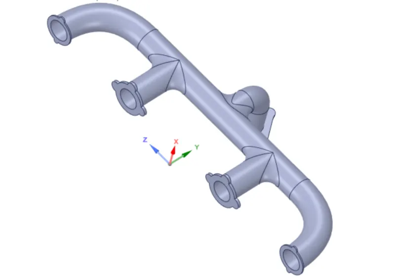
Fluid Volume (extracted by volume extraction option) -

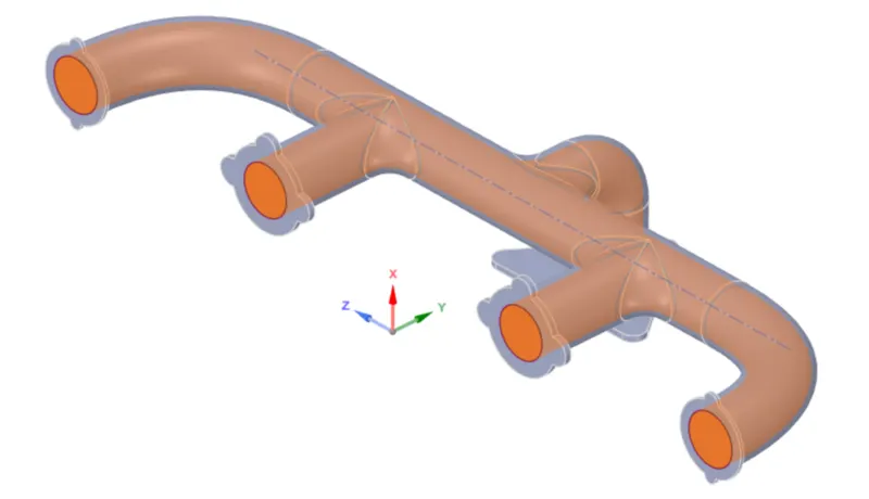
Solid Volume -

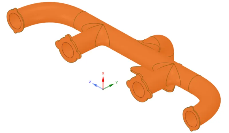
Finale Geometry (Including both the solid and fluid volume) -

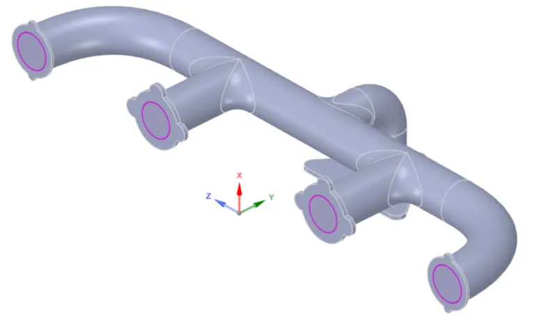
The purple line at the interface in the above model indicates that we have successfully achieved the share topology and hence we'll get a conformal mesh.

CASE 1 - Baseline mesh, K-epsillon method

Mesh -

The finale model is loaded into the mesh and first of all the named selections are created as shown below.

Named Selection -

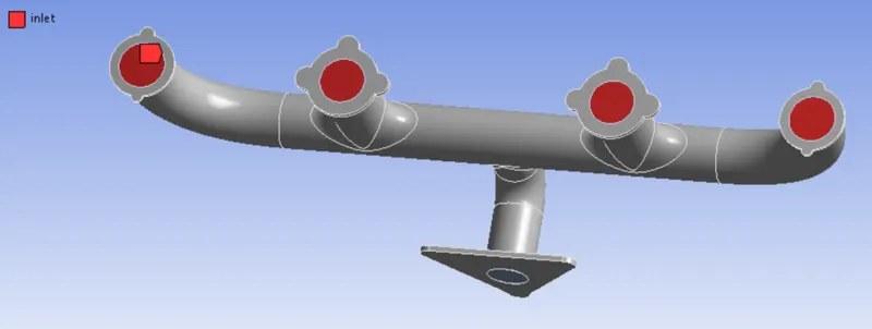
Inlet -

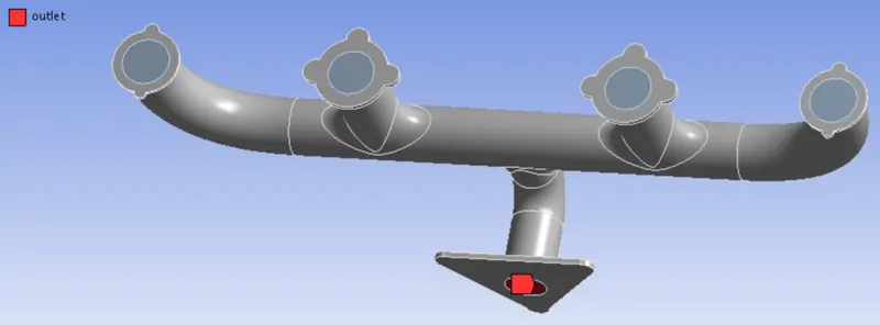
Outlet -

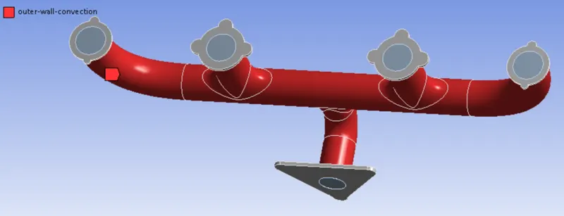
Outer Wall Convection -

Once we're done with the named selection, we can generate a base line mesh for our 1st simulation and after that we can keep refining the mesh for further simulations.

Base Line Mesh -

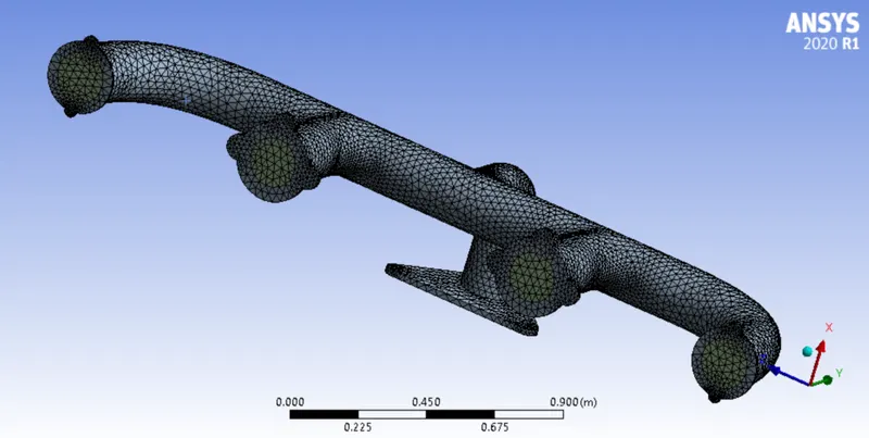
Element size - 150mm , no inflation layers.

In order to see if the mesh we have generated is accurate or not, we'll check a quantity known as orthogonal mesh quality which tells us about the quality of our mesh.

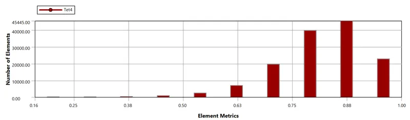
Number of Elements - 1,37,357

Setup -

The first thing we do is setup the boundary conditions which are given below.

• Inlet boundary condition

1. Type: Velocity inlet
2. Velocity magnitude: `5m/s`
3. Temperature: 700K

• Outlet boundary condition

1. Type: Pressure outlet
2. Gauge pressure: 0Pa

• Outer wall convection

1. Type: wall
2. Thermal condition: convection
3. Heat transfer coefficient: `20 W/(m^2K)`

The rest boundary condition values are set up as default values in ANSYS-FLUENT.

Material properties -

• Fluid -
  

  Material Name: Air

  Density: `1.225 (kg)/m^3`

  Specific heat: `1006.43 J/(kg*K)`

  Thermal conductivity: `0.0242 W/(m*K)`

  Viscosity: `1.7894e^-5 (Kg)/(m*s)`
  
  

• Solid -
  

  Material Name: Aluminum

  Specific heat: `871 J/(kg*K)`

  Thermal conductivity: `202.4 W/(m*K)`

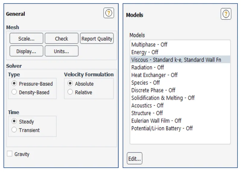
Energy equation is turned on and the Viscous model is set to k-epsilon model for this case as shown below.

Results -

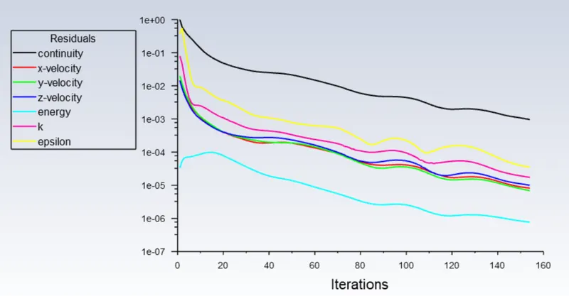
Residual Plot - (To check convergence)

Surface Heat Transfer Coefficient -

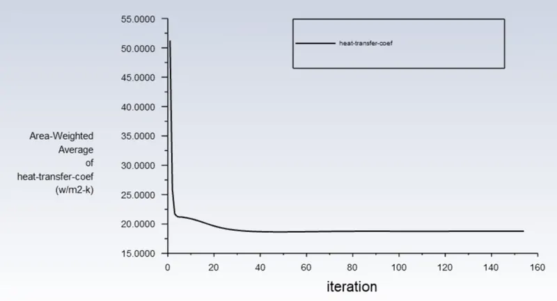
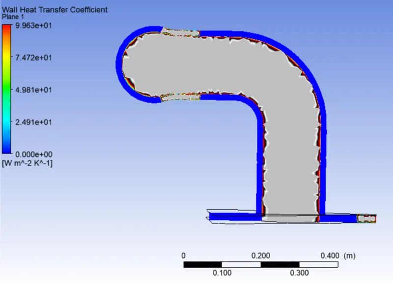
Surface Heat Transfer Coefficient - `18.779 W/(m^2K)`

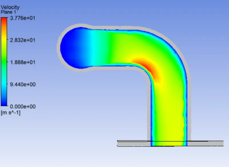
Velocity Plot -

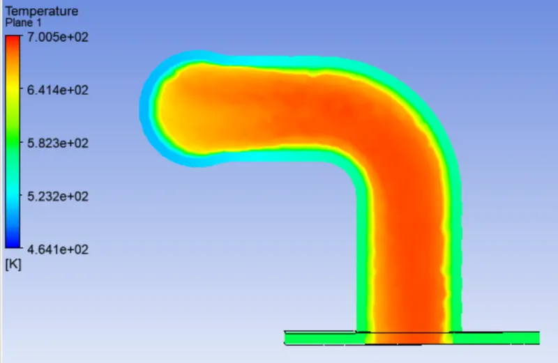
Temperature Plot -

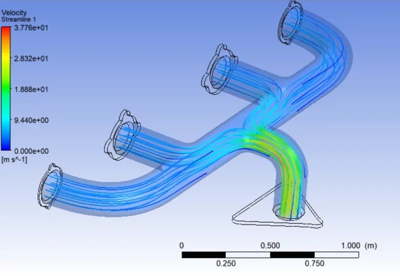
Velocity Streamline -

Wall Heat Transfer Coefficient-

Case 2 - Mesh refinement and using k-w SST model

Geometry -

Geometry is same as in the above case.

Mesh -

We'll refine our baseline mesh in order to improve the result. To refine the mesh the first thing we'll do is add inflation layers at the solid-fluid intersection and we'll also reduce the element size.

Refined Mesh -

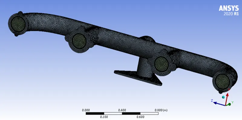
Element size - 15mm

Inflation layers - 12 layers, First layer thickness - 0.1732mm, `Y^+` - 3.

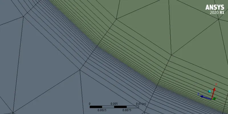
Mesh/Element Quality -

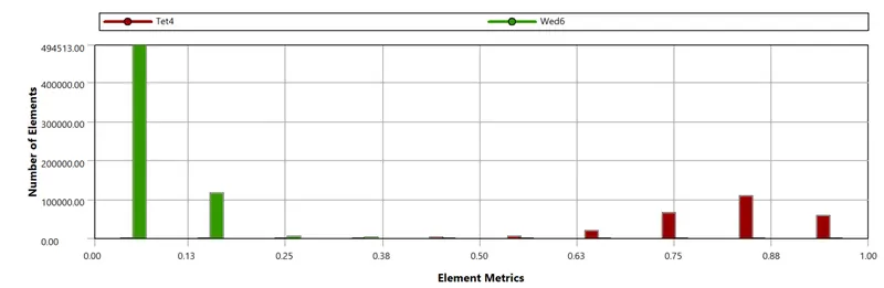
Numbe of Elements - 8,74,786

Setup -

Setup is same as in the above case, the only difference is that instead of using the k-epsilon model we'll use k-w(SST) model because this model is better in dealing with Y+ concept and hence will be useful in this case.

Results -

Residual Plot - (To check convergence)

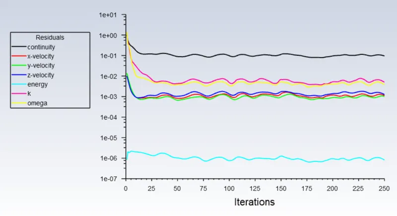
Surface Heat Transfer Coefficient -

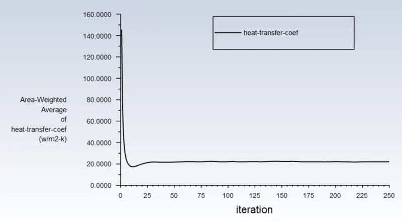
Surface Heat Transfer Coefficient - `21.004 W/(m^2K)`

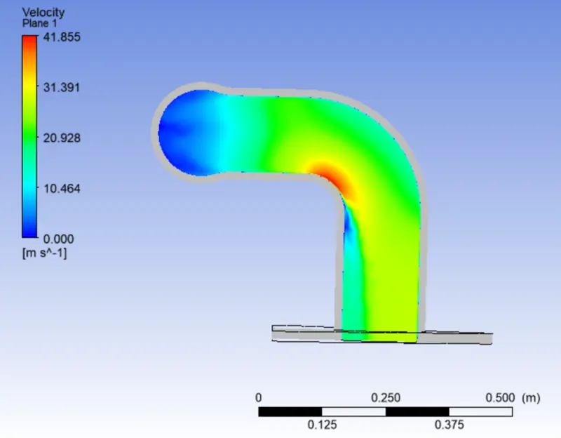
Velocity Plot -

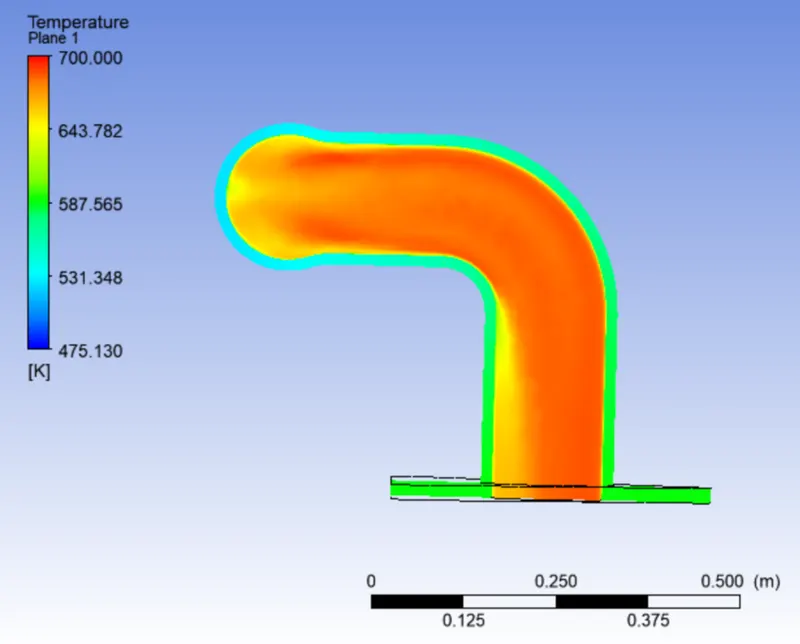
Temperature Plot -

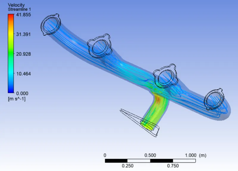
Velocity Streamline -

Wall Heat Transfer Coefficient-

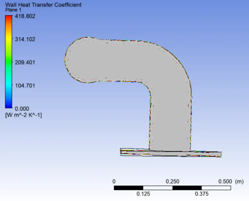
Case 3 - Finale Mesh refinement

Geometry -

Geometry is same as in the above case.

Mesh -

We'll refine our once again in order to improve the result.

Refined Mesh -

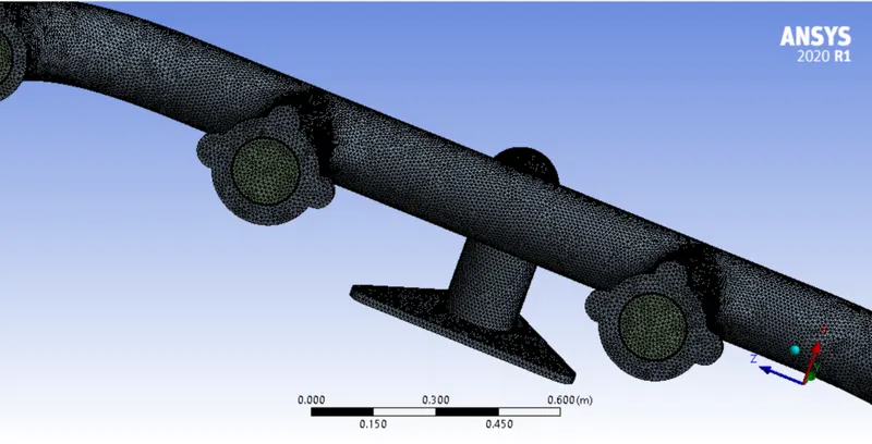
Element size - 10mm

Inflation layers - 12 layers, First layer thickness - 0.05776mm, `Y^+` - 1.

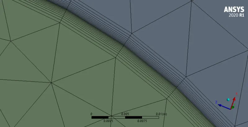
Mesh/Element Quality -

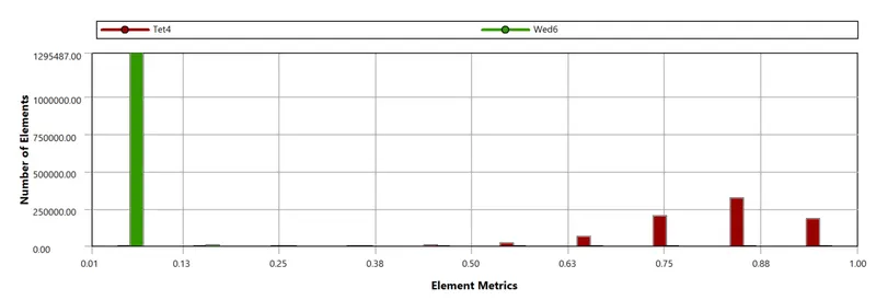
Number of Elements - 20,86,092

Setup -

Setup is same as in the above case.

Results -

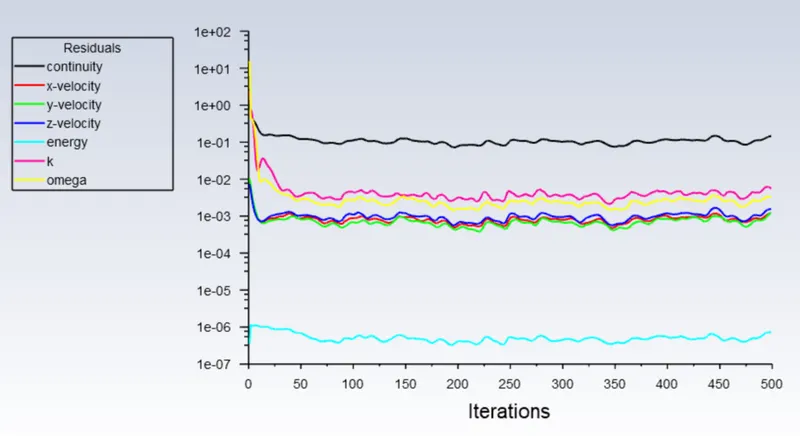
Residual Plot - (To check convergence)

Surface Heat Transfer Coefficient -

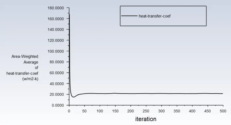
Surface Heat Transfer Coefficient - `20.380 W/(m^2K)`

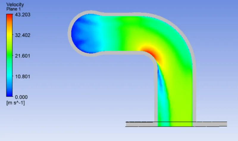
Velocity Plot -

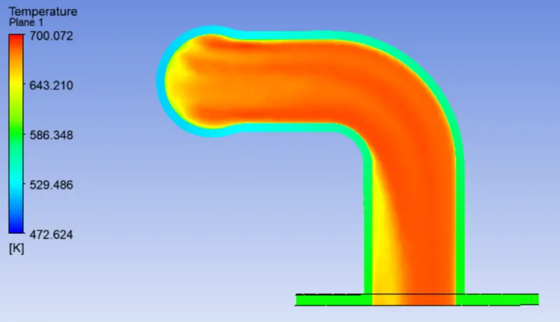
Temperature Plot -

Velocity Streamline -

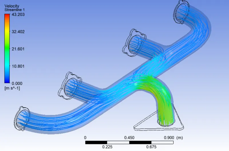
Wall Heat Transfer Coefficient-

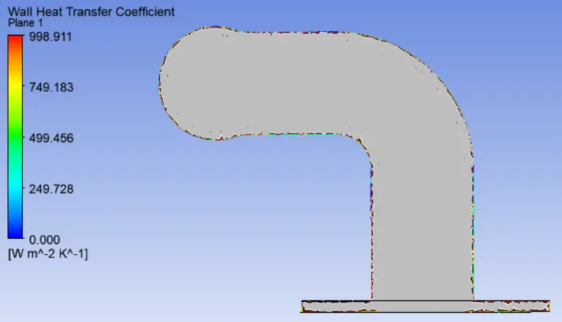
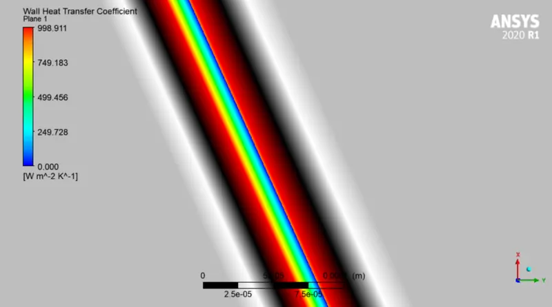
Close view of the fluid-solid interection layers -

Conclusion -

In order to verify if the HTC predictions from the simulations are right or not we'll have to compare our simulation results to the analutical solution and see how much error there is.

Analytical solution -

The Reynolds number for the given flow as calculated above is 58189.8960, which suggests that the flow is turbulent in nature, the Dittus Bolter heat transfer coefficient relation can be used to determine the Nusselt number which is described mathematically as

`Nu = 0.023Re^0.8Pr^0.4`

Where Pr is the prandtl number, For air at 700K the Prandtl number is Pr = 0.720

Hence, Nu = 131.502805

Since `Nu = (h*D)/k`

Where h = heat transfer coefficient, D = characteristic length = diameter of the exhaust pipe and k = thermal conductivity.

Therefore `h = (Nu*k)/D`

Hence `h =18.8198 W/(m^2K)`

Comparison table -

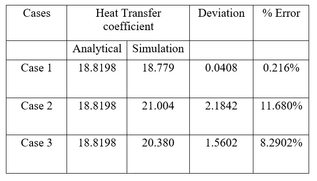
• The deviation of numerical heat transfer coefficient values from the analytical solution was found to be within 5 % to 10 % for the second and final mesh refinement are found to be in compliance with the industrial standards.
  
  
• The grid independence test was also observed during mesh refinement. Since the values for second the third case are near to each other, It is important that we limit ourselves to the second case only in order to save the computational time.
  
  
• The velocity at the outlet is higher than the velocity at the inlet can be attributed to the presence of four inlets and one outlet (Mass conservation).
  
  
• The accuracy of the heat transfer coefficient depends on selecting the suitable value of Y+ and type of turbulence model k – w(SST) vs k–epsilon model. The heat transfer coefficient values predicted by CFD simulation were validated against the analytical solution and the deviations observed were in the range of 5 % to 10 % which is in compliance with industrial standards. However, the accuracy of k - wSST model itself depends on the accuracy of the analytical solution (finding the right Y+ value), flow properties, and geometry.
  
  
• The values predicted by the baseline mesh and the refined mesh were close to each other this can be attributed to the fact that the boundary keeps on growing from the inlet and starts declining to as it moves towards the outlet owing to change in velocity, thus the value is predominant at the outlet section of the exhaust port.