Week 4 - CHT Analysis on Exhaust port

Aim: To Perform Conjugate Heat Transfer analysis on a given geometry of Exhaust port.

Theory:

1. Conjugate Heat Transfer (CHT) Analysis :
   Whenever there is a heat transfer through solids and fluids simultaneously, the approach of solving the problem case through a set of transport equations on the basis of materials and given boundary conditions is known as the conjugate heat transfer (CHT) analysis.
   The conduction is the dominant mode of heat transfer in solids while in fluids the convection is the dominant mode of heat transfer.
   
   Heat Transfer in solids and fluids is combined in the majority of applications. As the solids are generally immersed in fluids the Conjugate Heat Transfer (CHT) analysis is very helpful in predicting the temperature distribution and heat transfer rates and their effects.
   
   Conjugate Heat Transfer approach does not require beforehand knowledge of heat transfer coefficients for given problem, on the basis transport properties and material properties the heat transfer coefficients for any system of heat transfer coupling can be predicted by setting the right case.
   
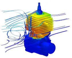
   Examples of conjugate heat transfer are various heat exchangers like coolers, heaters , condensers, evaporators, Plate heat exchangers (PHE) etc. ; CHT is observed in natural and forced convection cases , at fluid solid interfaces where energy is being transferred. Also in the case of radiative heat transfer and PCM based thermal energy storages the CHT phenomenon is observed. [1]
   
   

   	Shell and Tube Heat Exchanger		Air cooling in Engine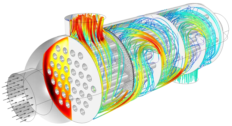
   	Cooling of Electronic components using heat sink		Plate Type Heat Exchanger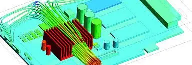
   	Images Source: Google.

   
   
   
2. Selection of Turbulence Model and y plus value.
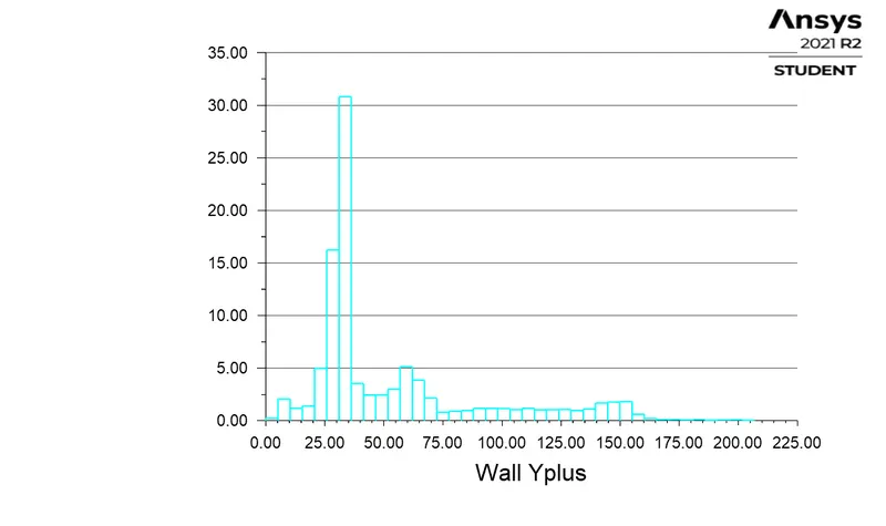
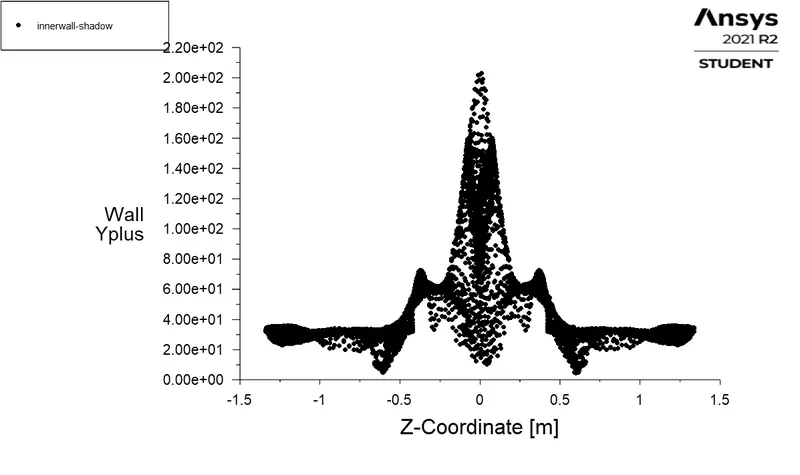
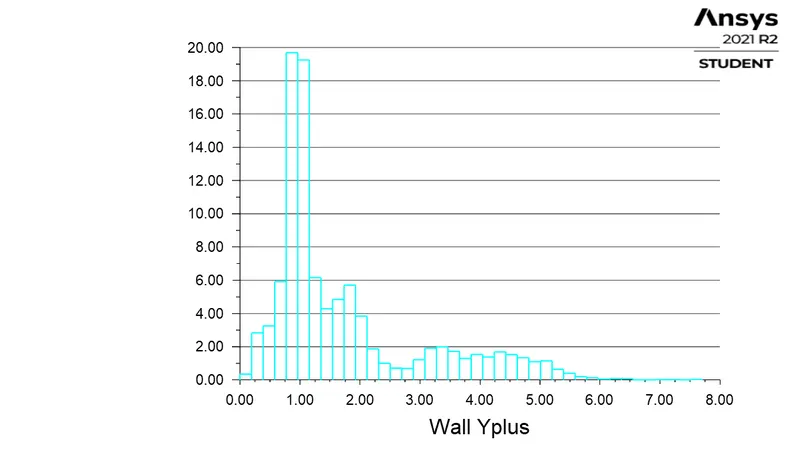
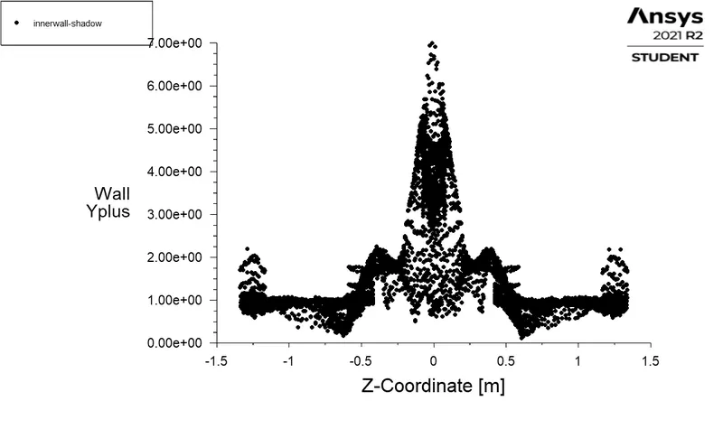
   Here both k-epsilon and k-omega SST turbulence models can be used for the CHT analysis of a given geometry of the exhaust port. For the k-epsilon model the comparatively coarse mesh can be used with y+ value between 30 to 300. While for the k-omega SST turbulence model the refined mesh must be used with y+ value of 1 to 5.
   
   
3. Calculation of heat transfer coefficient(HTC)
   For a steady state, the Heat transfer rate from hot exhaust gas to the inner wall of the exhaust port body must be equal to the Heat transfer rate from outer wall of exhaust port body to the surrounding air at ambient temperature.
   
   Heat Transfer rate from exhaust gas to inner wall of exhaust port body is,
   ` (dotQ)_("in") = h_g * A_("in")*(T_g - T_("win"))`;
   Heat Transfer rate from exhaust port inner wall to outer wall is,
   ` (dotQ)_w = (2*pi*L_(ex)*k_w *(T_("win") - T_(wo)))/(ln(D_o / D_"in"))`;
   Heat Transfer rate from outer wall of exhaust port body to surrounding is,
   ` (dotQ)_o = h_o * A_(o)*(T_(wo) - T_a)`;
   
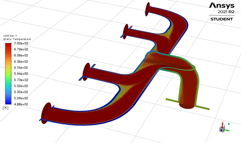
   As exhaust port wall material has high thermal conductivity and the wall thickness is very small the inner and outer wall temperature should have negligible difference. i.e. the Temperature drop across the exhaust port wall is negligible and thus the inner and outer wall temperature should be considered as same.
   
   This is depicted in the network of thermal resistances as follows: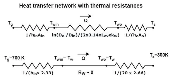
   
   
   
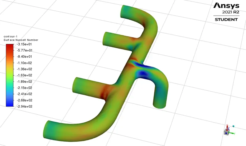
   Thus the heat transfer rate and exhaust port wall temperature is known then value of heat transfer coefficient for hot exhaust gas to inner wall of exhaust port body can be calculated and same can be verified with the one obtained with the appropriate established correlation formula for the same case.
   
   
   
4. The correlation to obtain heat transfer coefficient for fully developed internal turbulent flow through smooth pipes is given by `"Dittus-Boelter Equation"` .
   
   `"Dittus-Boelter Equation"` - `Nu = 0.023 * (Re)^0.8 * (Pr)^n `
   where, ` n = 0.4 ` - for fluid being heated ;
   & ` n = 0.3 ` - for fluid being cooled .
   (Error can be as great as 25%) [2]
   
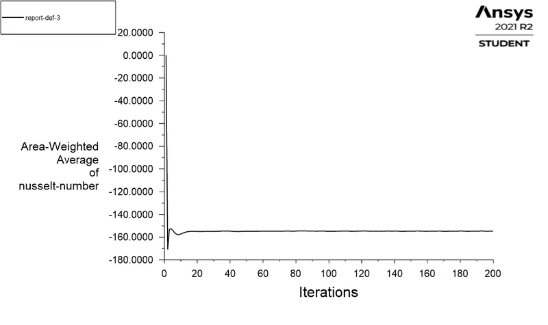
   Here fluid is being cooled thus `Nu = 0.023 * (Re)^0.8 * (Pr)^0.3 ` is applicable and value of heat transfer coefficient is obtained by ` h = (Nu * k_f )/ L_c ` where symbols have their usual meanings.
   Exhaust gas properties are assumed to be the same as that of air.
   
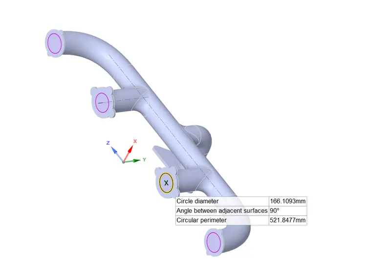
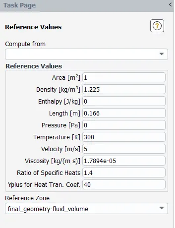
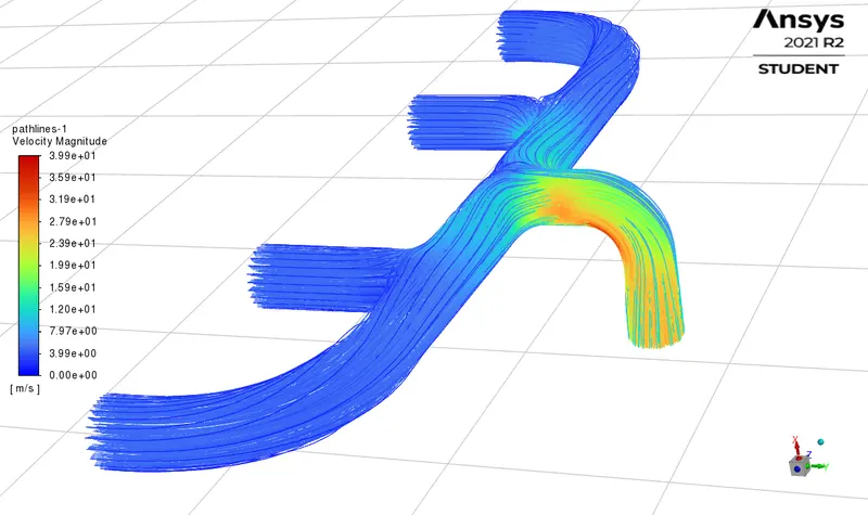
   At inlet `v =5 m/s` and inlet diameter `D_"inlet" = 0.166 m` thus `Re = (rho * v *D_"inlet" ) / mu = 56821` which is greater than 2300 thus flow is turbulent.
   Also for air `Pr =0.71 ` at 700 K .
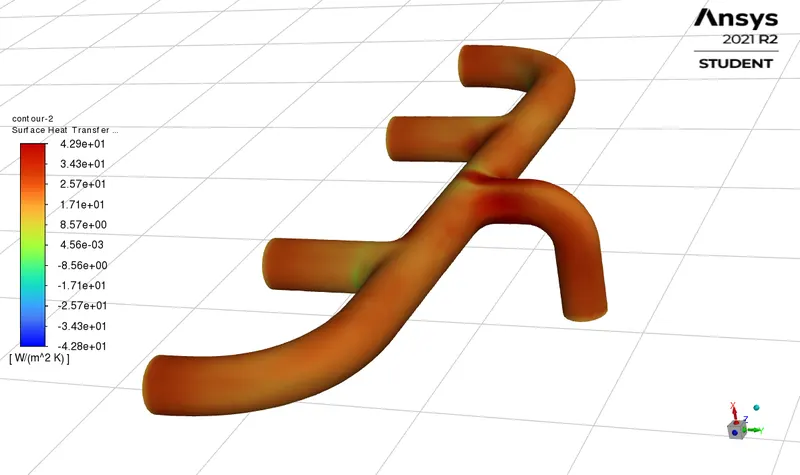
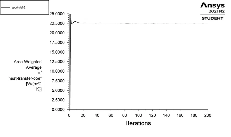
   Thus ` Nu = 0.023 * (56821)^0.8 * (0.71)^0.3 = 132.04 ` and `h_"in" = 19.25 W/(m^2 * K)` .
   
   
5. Velocity of exhaust gas at outlet can be theoretically calculated using continuity equation as follows,
   as the density of exhaust gas is going to be constant throughout the exhaust port and inlet and outlet are circular in crosssection with 4 number of inlets and 1 outlet, then continuity equation becomes
   `4*(D^2 * V)_"inlet" = (D^2 * V)_"outlet"`
   
   i.e. `V_"outlet" = (D^2 * V)_"inlet" / (D^2)_"outlet"
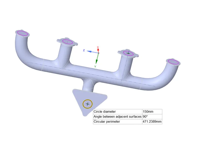
   = (4*(0.166)^2*5)/(0.15)^2
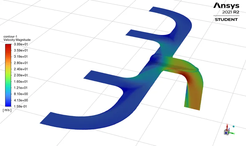
   = 24.494 m/s` .

Workflow:

1. Exhaust Port Geometry:
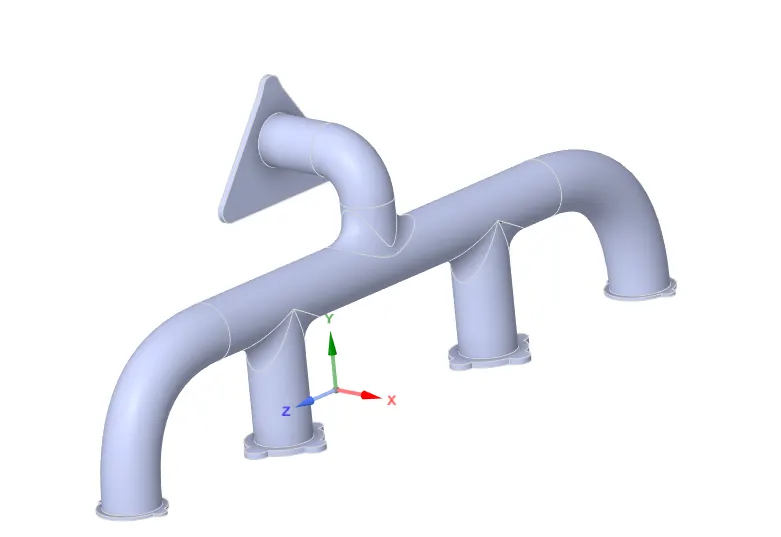
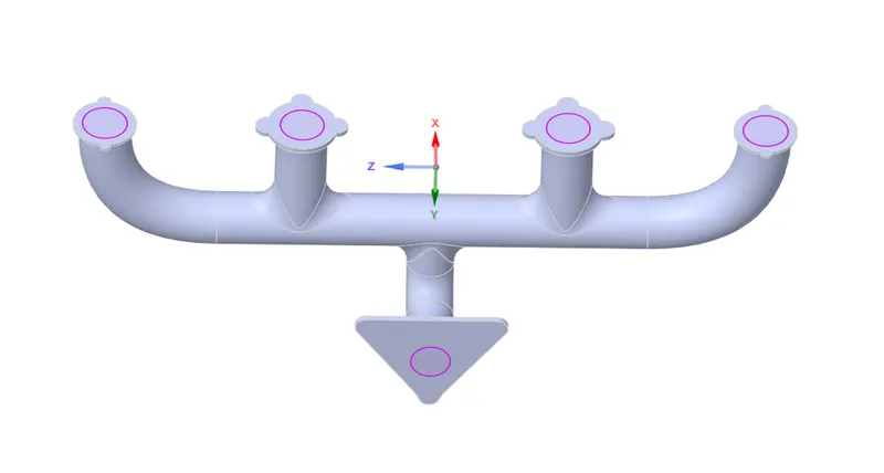
   The provided geometry model is imported into the spaceclaim and fluid volume is generated. The dimensions measured for inlet and outlet diameter as those will be needed for calculations.
   
   
   
   
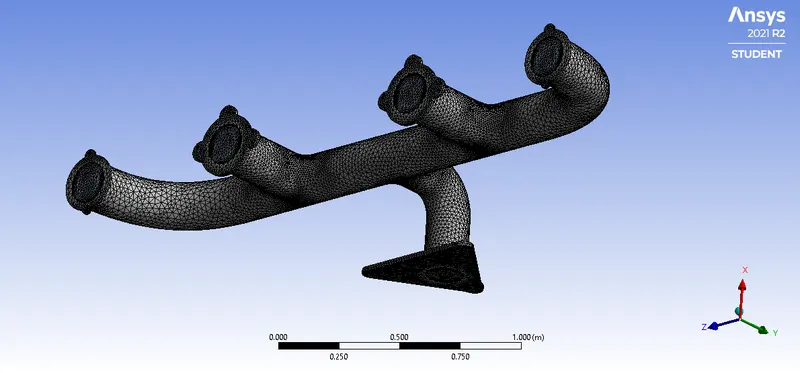
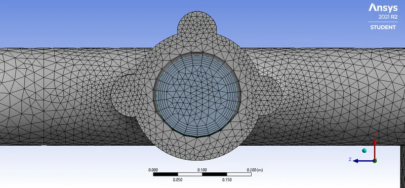
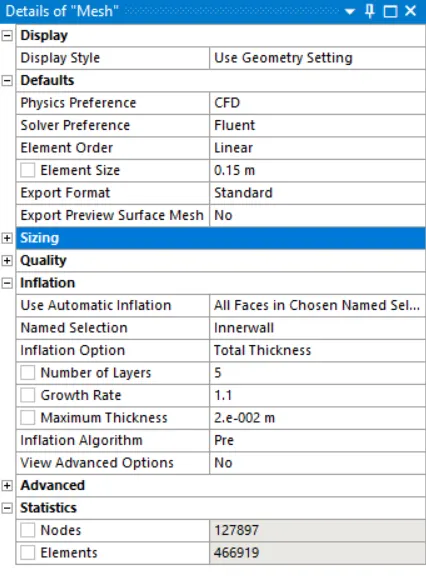
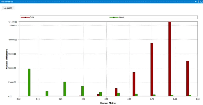
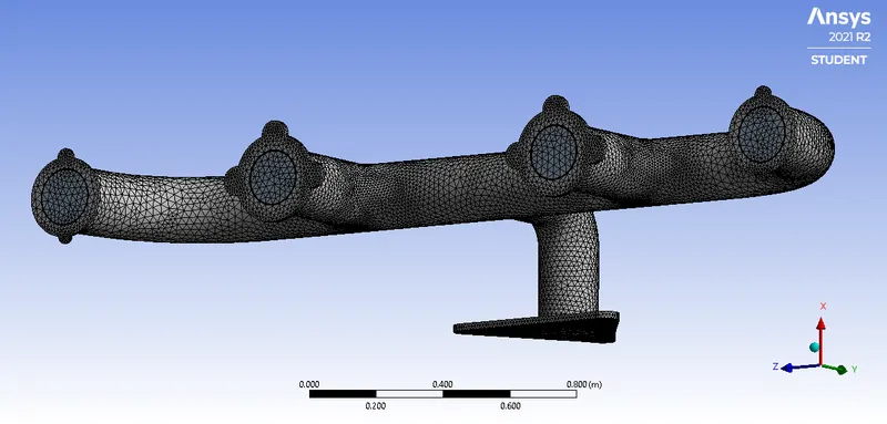
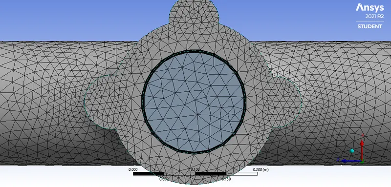
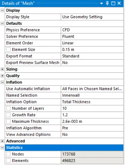
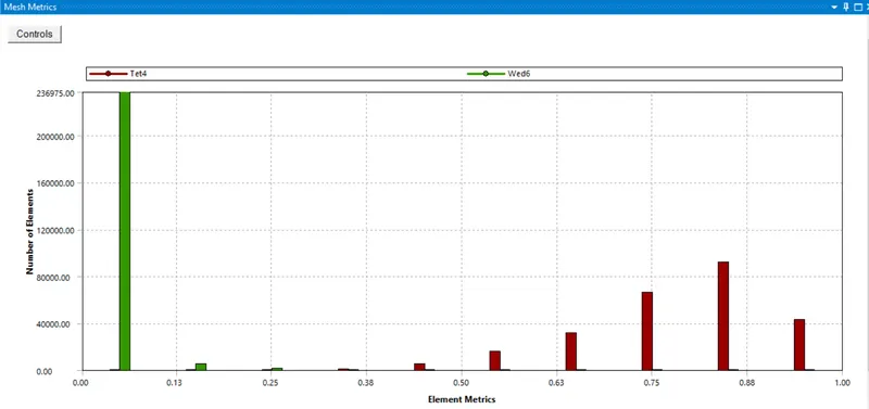
2. The prepared geometry model with shared topology is imported into the Meshing tool where after assigning the named selections the geometry is meshed as per the requirements. The inflation layer thickness has been given according to the required y+ value as per the turbulence model being used for analysis. The Mesh Metrics chart is provided for mesh elements quality.
   
   
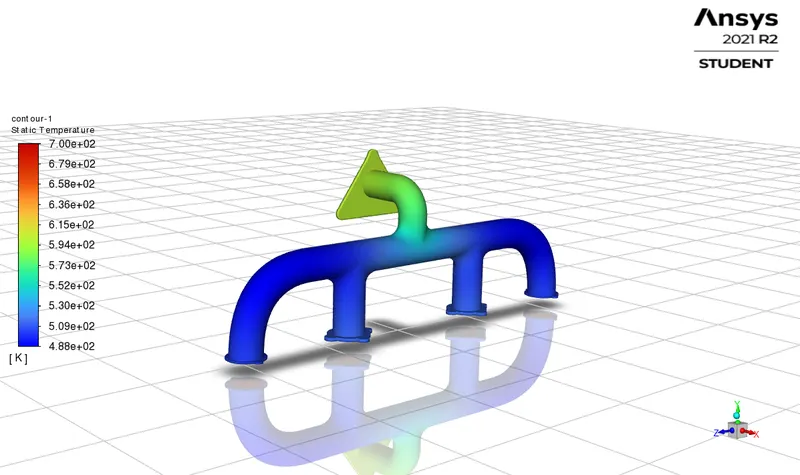
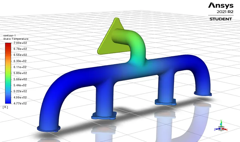
3. The Mesh is imported into the fluent , turned on the Energy Model. The required turbulence model is selected. In Materials, for solid aluminium is selected while for fluids air is selected. Velocity inlet type boundary is assigned to all four inlets whereas the pressure outlet type boundary condition is assigned to the outlet. The outer wall of the exhaust port is assigned with convection type boundary condition with convection heat transfer coefficient of 20 W/(m^2 *K) with surrounding air at a temperature of 300 K .
   
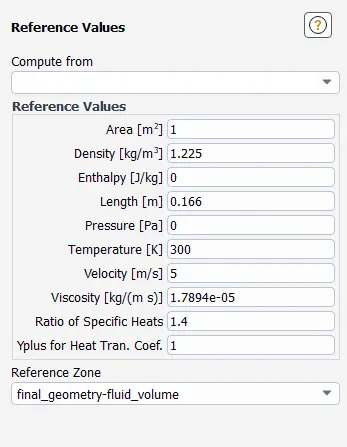
4. The necessary reference values have been set accordingly.
   
   
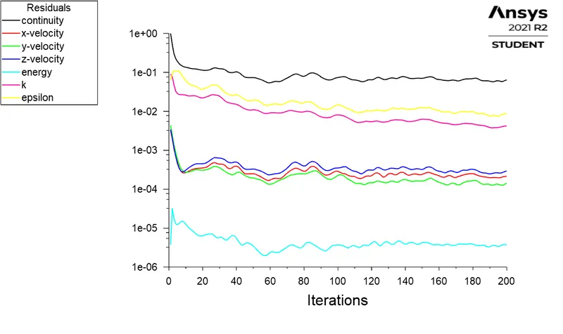
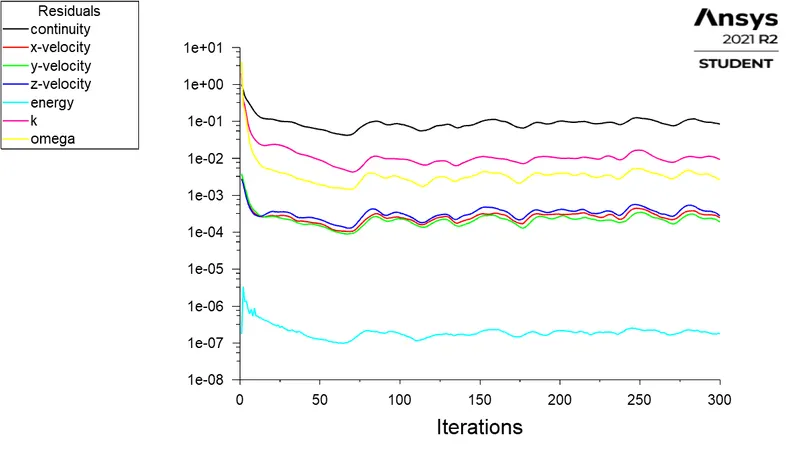
5. The Coupled Solution scheme has been selected and residual limits are set, also the required monitoring plots and contours are set prior to initialising the solution then the animations setting are done. Then after giving the number of iterations the solution has been calculated.
   
   
6. The solution results are analysed for convergence and accuracy. Same has been validated with the reference data / steady state solution.
   
   
7. For this CHT analysis both of turbulent models i.e. k-epsilon and k-omega SST, have been used in separate cases and results are analysed for accuracy.

Case I :

	Turbulence Model : k-epsilon y+ = 40			Inflation layer total thickness = 20 mm; Number of inflation layers =5 ; Growth rate =1.1 .
	Mesh			Inflation layers
	Mesh Details			Mesh Metric
	Residual Plot			Reference Values
	Temperature contour on outer wall convection			Temperature contours on cross sectional planes
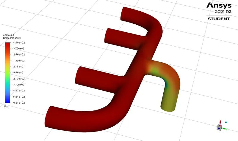
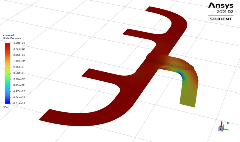
	Pressure contour on inner wall shadow			Pressure contours on cross sectional planes
	Velocity Streamlines through the fluid domain			Velocity contours on cross sectional planes
	Surface heat transfer coeff on inner wall			Plot of Surface heat transfer coeff on inner wall
	Nusselt Number contour on inner wall-shadow			Plot of Average Nusselt Number on inner wall-shadow
	y+ Histogram			y+ along Z-coordinate
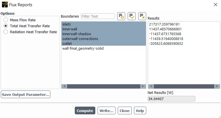
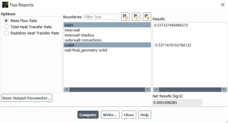
	Heat Flux balance			Mass flow balance
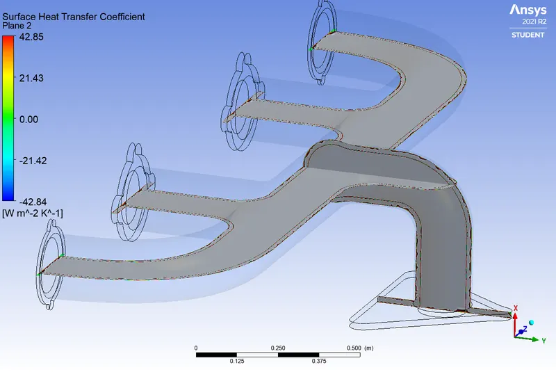
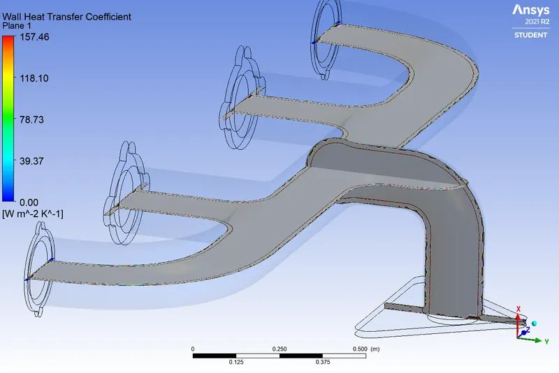
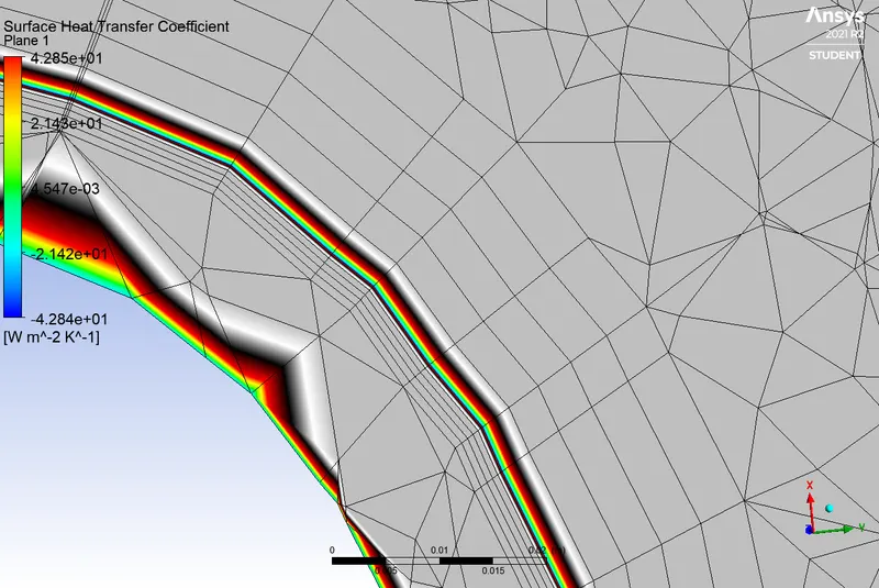
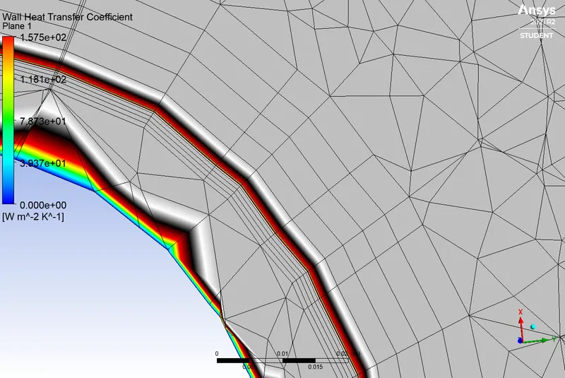
	Surface Heat Transfer Coefficient on cross sections			Wall Heat Transfer Coefficient on cross sections
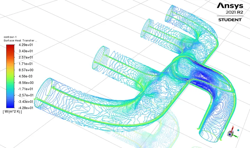
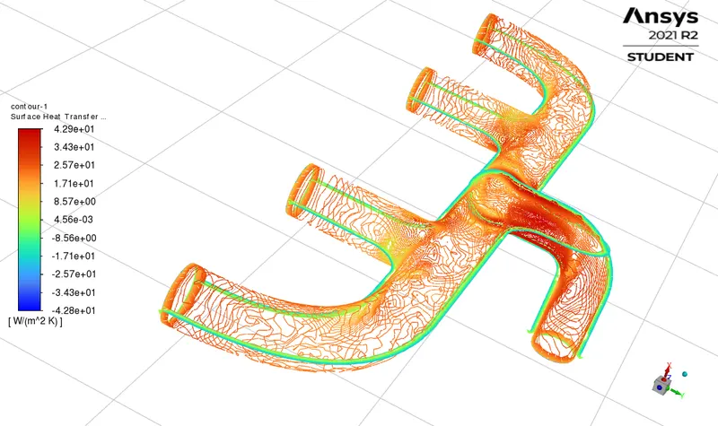
	Surface Heat Transfer Coefficient contour on innerwall-shadow			Surface Heat Transfer Coefficient contour on innerwall
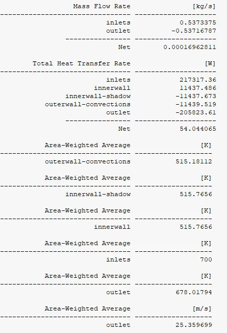
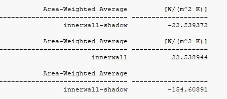
	Console Output for various parameters			Console Output for various parameters

Case II :

	Turbulence Model : k-omega SST y+ = 1			Inflation layer total thickness = 2.6 mm; Number of inflation layers =10 ; Growth rate =1.2 .
	Mesh			Inflation layers
	Mesh Details			Mesh Metric
	Residual Plot			Reference Values
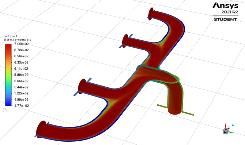
	Temperature contour on outer wall convection			Temperature contours on cross sectional planes
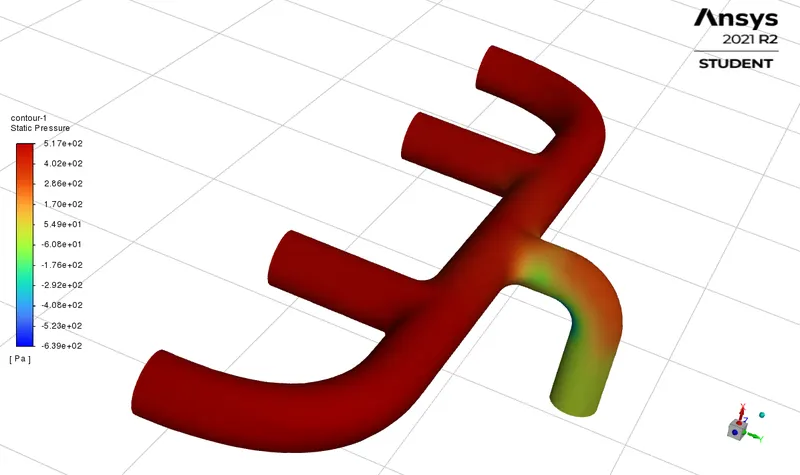
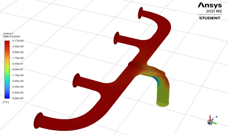
	Pressure contour on inner wall shadow			Pressure contours on cross sectional planes
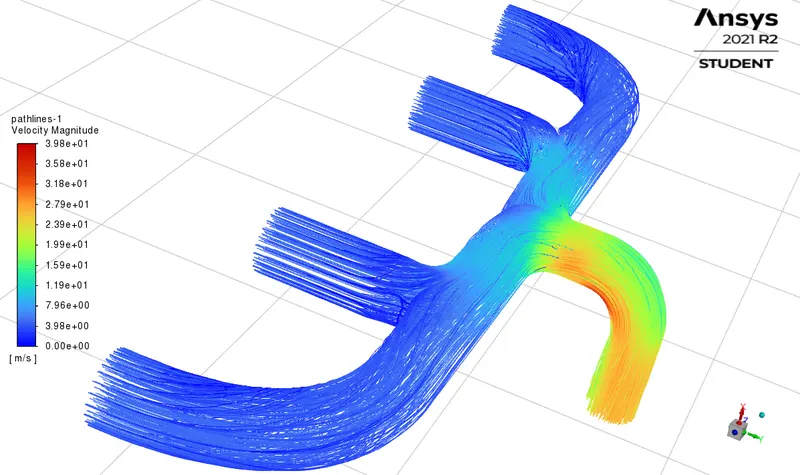
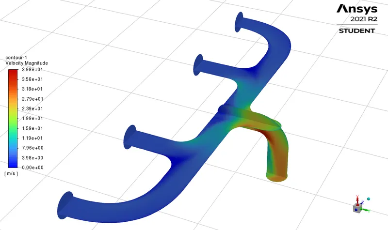
	Velocity Streamlines through the fluid domain			Velocity contours on cross sectional planes
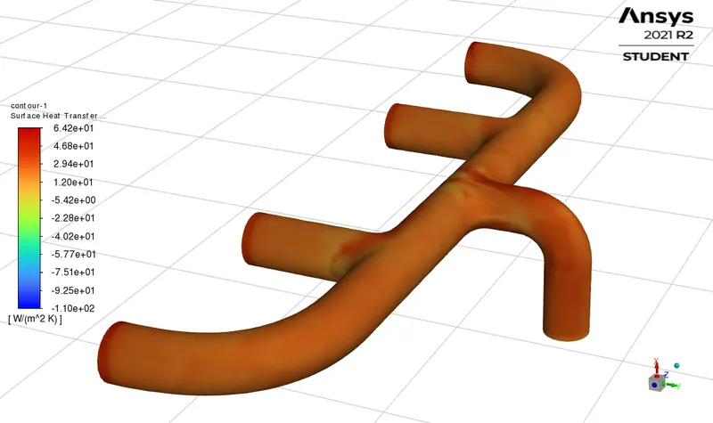
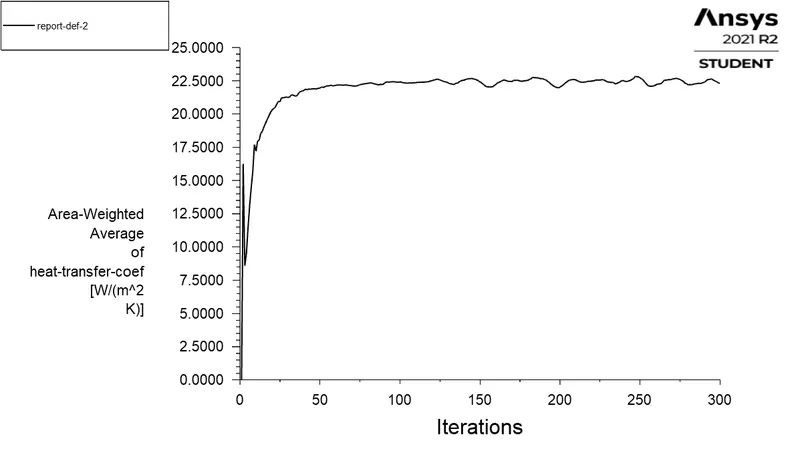
	Surface heat transfer coeff on inner wall			Plot of Surface heat transfer coeff on inner wall
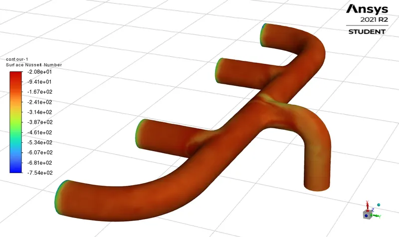
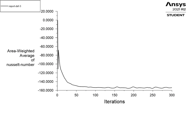
	Nusselt Number contour on inner wall-shadow			Plot of Average Nusselt Number on inner wall-shadow
	y+ Histogram			y+ along Z coordinate
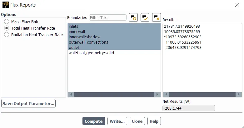
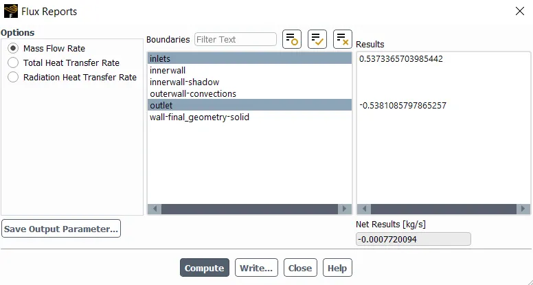
	Heat Flux balance			Mass flow balance
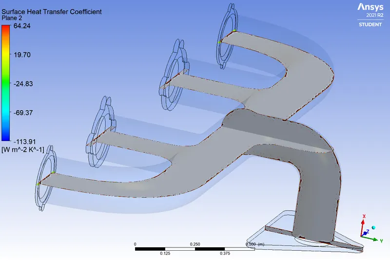
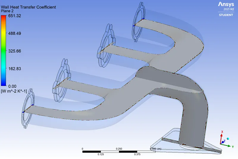
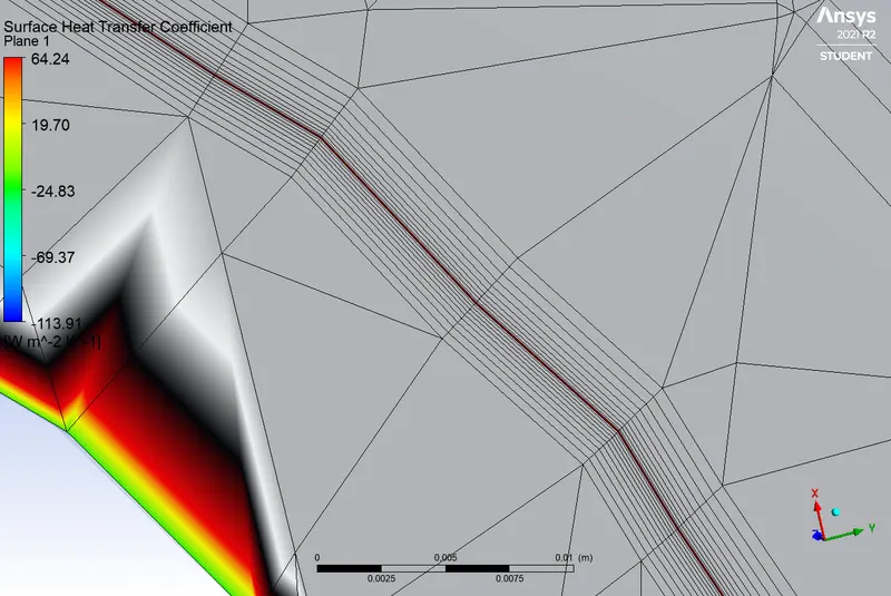
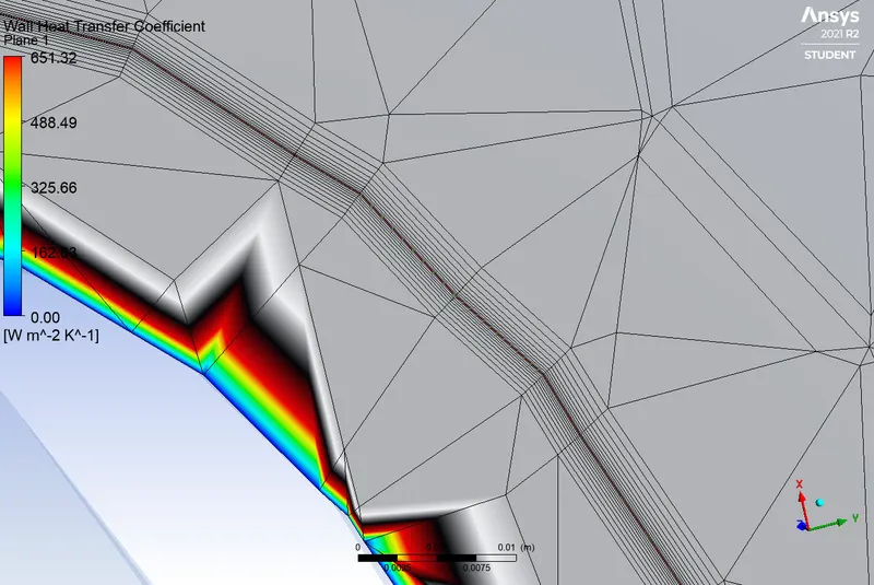
	Surface Heat Transfer Coefficient on cross sections			Wall Heat Transfer Coefficient on cross sections
	Surface Heat Transfer Coefficient contour on innerwall-shadow			Surface Heat Transfer Coefficient contour on innerwall
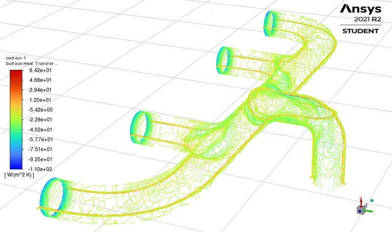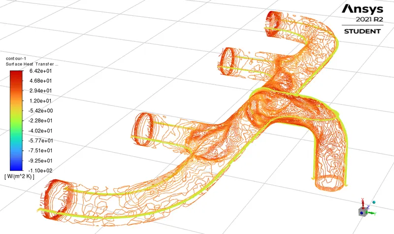	Console Output for various parameters			Console Output for various parameters

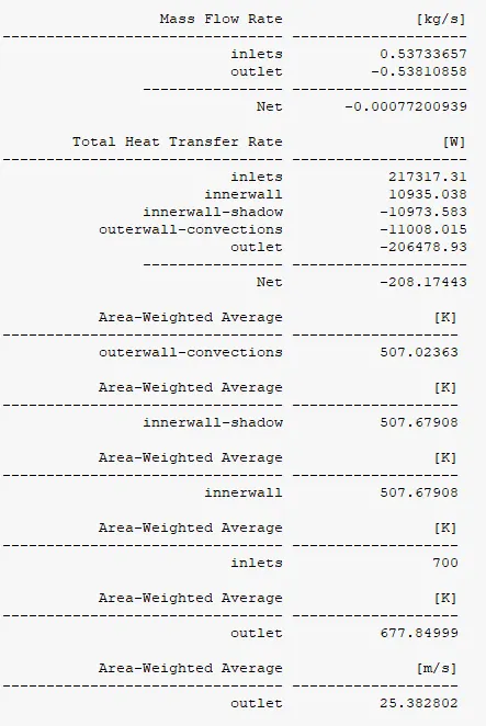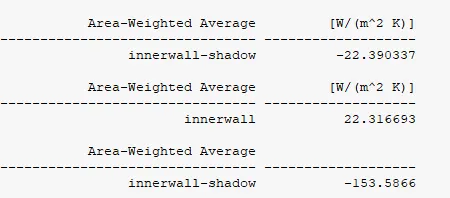Observation Table:

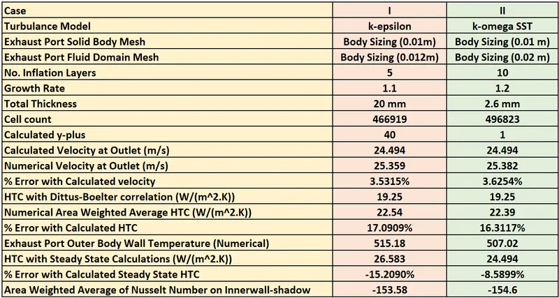
Results and conclusions:

1. From the Observation Table it is clear that errors for Heat Transfer Coefficients are comparatively marginally greater in case of k-epsilon turbulence model than the case of k-omega turbulence model.
2. The results from both cases are within the acceptable range of tolerances, thus can be accepted.
3. The numerically obtained values of heat transfer coefficients are compared with the values obtained with established correlation (Dittus-Boelter equation) and errors observed are within the specified range for the correlation.
4. The numerically obtained values of heat transfer coefficients are also compared with the calculated steady state heat transfer coefficients with the help of numerically obtained outer wall temperatures.
5. By comparing the numerical heat transfer coefficients with the values obtained from correlation and steady state calculations the results are justified with acceptable errors.
6. Errors with heat transfer coefficients obtained by correlation are on the higher side due to the values of air properties used to evaluate the same and for simulation the same properties are considered constant.

References:

1. https://www.comsol.com/blogs/conjugate-heat-transfer/
2. Heat and Mass Transfer book by Y Cengel. (Page no. 460)