Week 4 - CHT Analysis on Exhaust port
Objective: observing the thermal behavior of hot fluid flowing through the exhaust pipe, and obtaining an accurate value of the heat transfer coefficient on the internal solid surface on the exhaust manifold.
Introduction
Conjugate heat transfer analysis is used to capture accurate heat transfer behavior due to both convection and conduction, for cases in which a solid and fluid at different temperatures are subjected to different thermal conditions interact with each other. This is especially useful at the fluid solid interface, where the fluid interacts thermally and solid. The result obtained is a coupled solution, taking into account the thermal effect due to both, conduction and convection. It is also known for its flexibility, and its ability to handle complex simulations. Conjugate heat transfer can be used in wide range of cases that involves mass flow of slide over or inside a solid, subjected to different thermal conditions. Examples of the uses of CHT is seen in the determination of the effectiveness of heat transfer of a solid fin with a fluid flowing around it, fluid flowing through a tube at a different temperature, such as a heat exchanger, and many more applications. A point to note is that CHT is not limited to just conduction and convection, but can take into consideration radiation heat transfer as well.
In this particular case, the hot fluid flowing through the exhaust pipe is air, at 427 degrees Celsius. The Hartford interacts with the solid surface of the pipe, which is at a lower temperature, and the heat transfer at this point is due to convection. The inner wall in contact with the fluid increases the temperature, and the head then flows from the inner wall to the outer wall. The pipe thickness is heated, caused by heat transfer due to conduction. The outer wall of the exhaust pipe is subjected to convection at 20 `W/m^2`at 30 degrees Celsius.
Theory
The exhaust manifold is a vital component in automotive design of a vehicle, as it is used to collect the exhaust gases formed due to combustion of the fuel and air within the cylinders, and provide a path for the gases to escape to the atmosphere. The exhaust manifold has multiple inlets connected to the exhaust port on the cylinders in the engine. The high-pressure exhaust gases flow through the pipe with relative ease. As the pressure difference between the exhaust pipe outlet and atmospheric pressure and the high-pressure exhaust gases in the cylinder is enough for the gases to get sucked out of the combustion chamber.
CASE SETUP
Geometry creation
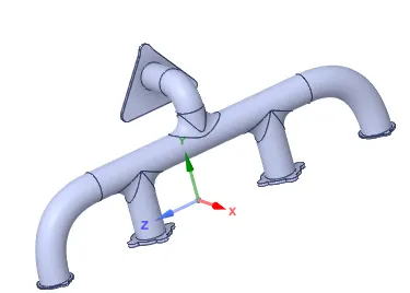
- Import cad design in SpaceClaim.
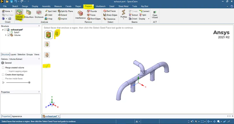
- Extract volume
- extracted volume.
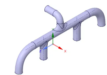
- extracted volume.
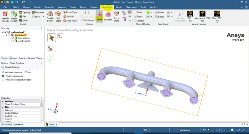
- Share topology to make sure that generated mesh is conformal mesh.
Meshing
- Create a baseline mesh.
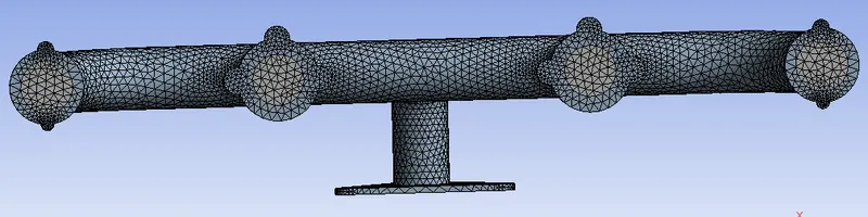
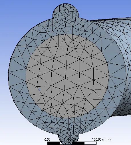
- Near wall mesh.
- Named selection
- Select the faces to name it.
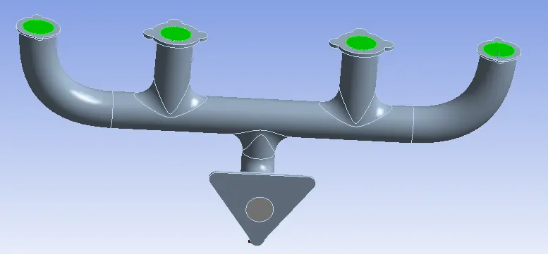 nsert
nsert 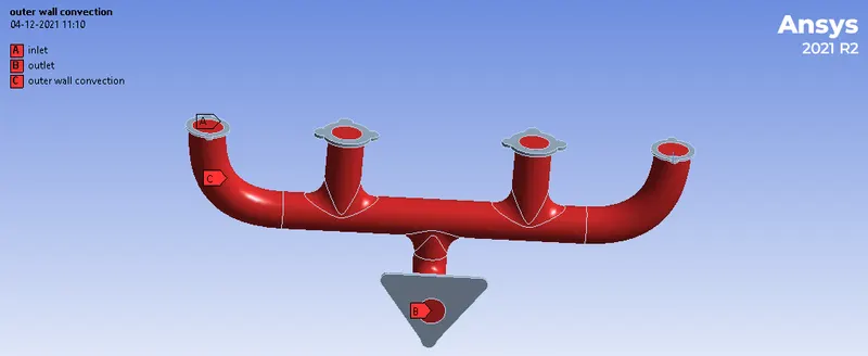
- Select the faces to name it.
Mesh refinement
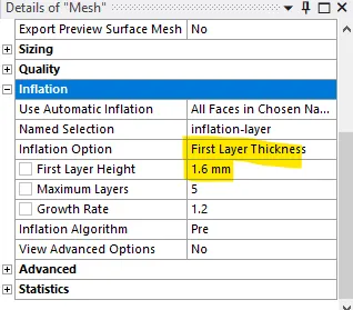
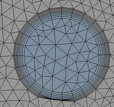
- Insert inflation layer using appropriate first layer thickness, based on the calculation of Y+ range for the particular turbulence model.
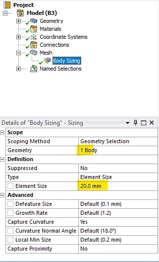
- insert body sizing and select slid volume for the geometry.
Ansys setup
- Physics setting.
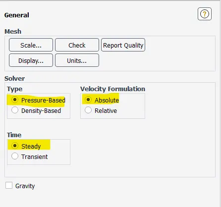
- Solver type : Pressure Based.
- Velocity formulation : absolute
- Time : steady state
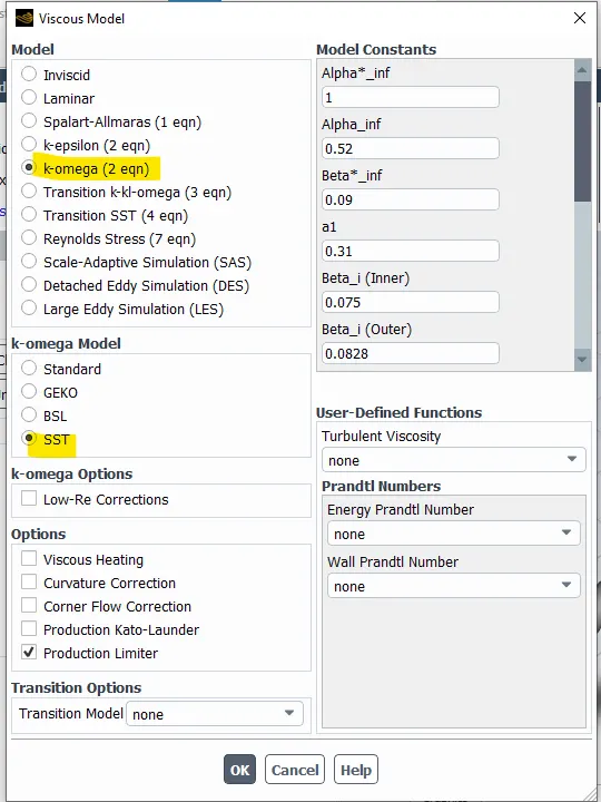
- Turbulence model: K-omega SST model.
- The k-Omega SST model has been designed to combine the advantages of the k epsilon and k-omega turbulence model. The k-Omega model shops the near wall functions accurately, but is inaccurate in the free stream velocity section of the fluid flow whereas the K-epsilon model accurately solves the free stream section of the fluid flow, but provides inaccurate values at the near wall or viscous sublayer suction.
- The k Omega SST model uses of K-epsilon model in the free stream section of the fluid flow, and lucky Omega model for near v competitions. The ability of the k-omega SST model to resolve near wall behavior is imperative to attend precise thermal behavior near the inner wall.
- This seamless switching between models is done by the integration of two blending function F1 and F2 in the equations of a specific dissipation rate and kinematics Eddy viscosity respectively.
- If the value of F1 is zero, the model switches to the k-epsilon model, similarly if the value of F1 is 1. the k- Omega model is used.
- F2 involves the use of viscosity limiter, which prevents the model from over predicting the wall shear stress, and functions similar to F1.
- Turbulence model: K-omega SST model.
- Turbulence model: K-`omega` SST model.
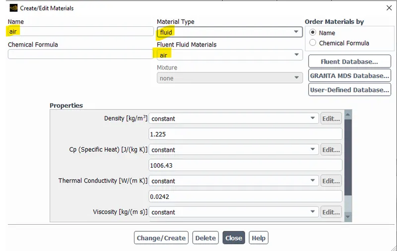
- Material selection.
- fluid: Air
- Solid: Aluminum
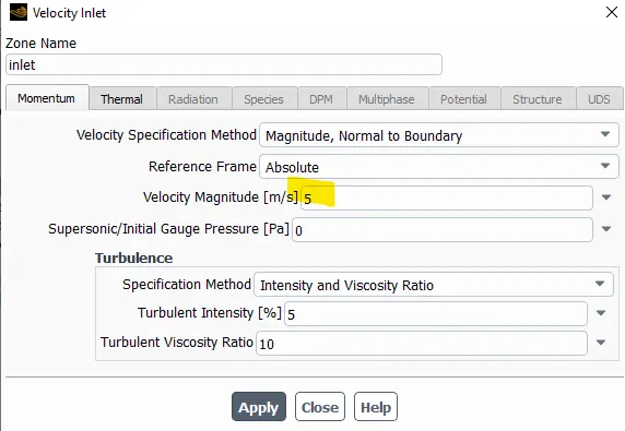
- Change boundary conditions.
- Inlet
- Velocity: 5m/sec.
- Temperature: 700K.
- Outer wall convection
- Heat transfer coefficient: `20W/(m^2.K)`
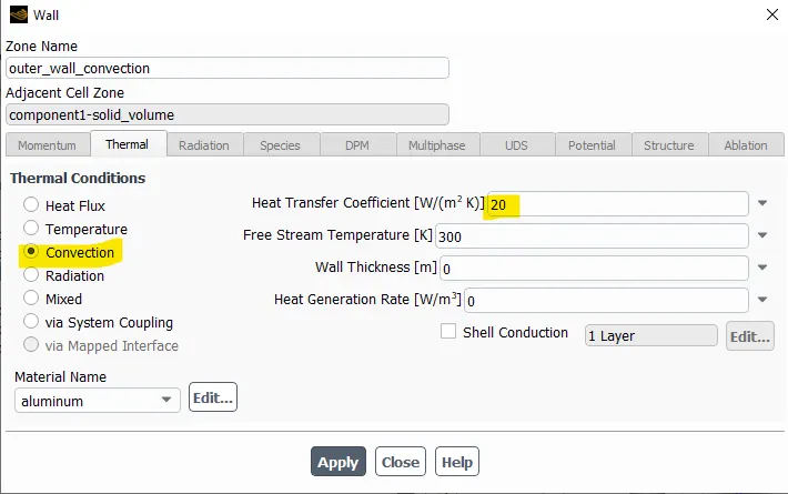
- Heat transfer coefficient: `20W/(m^2.K)`
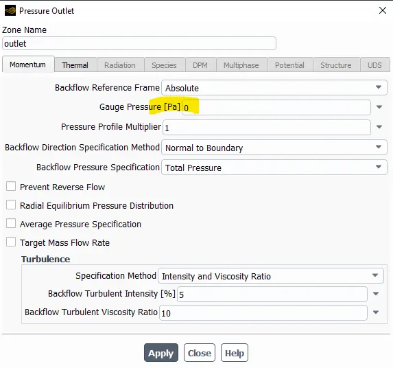
- Outlet: pressure outlet at zero-gauge pressure.
- Inlet
- Create a report definition for the surface heat transfer coefficient.

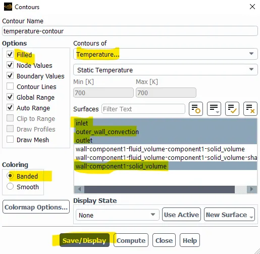
- create a temperature contour.
Post processing results
FOR BASELINE MESH
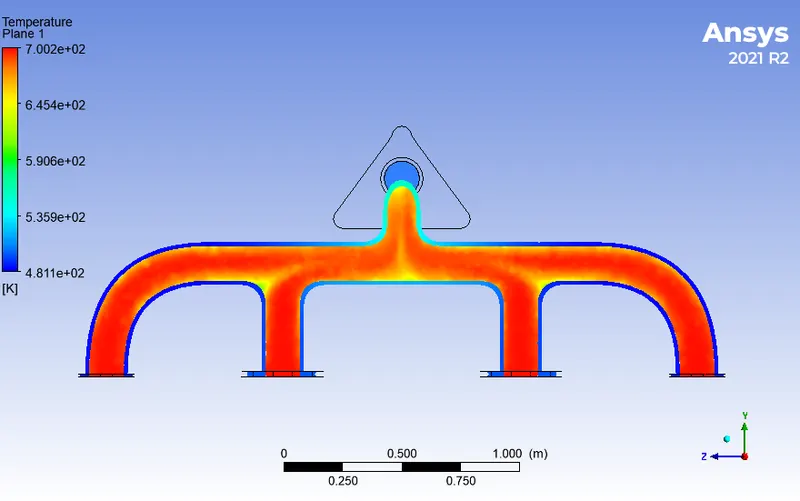
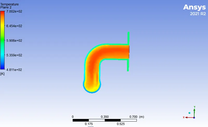
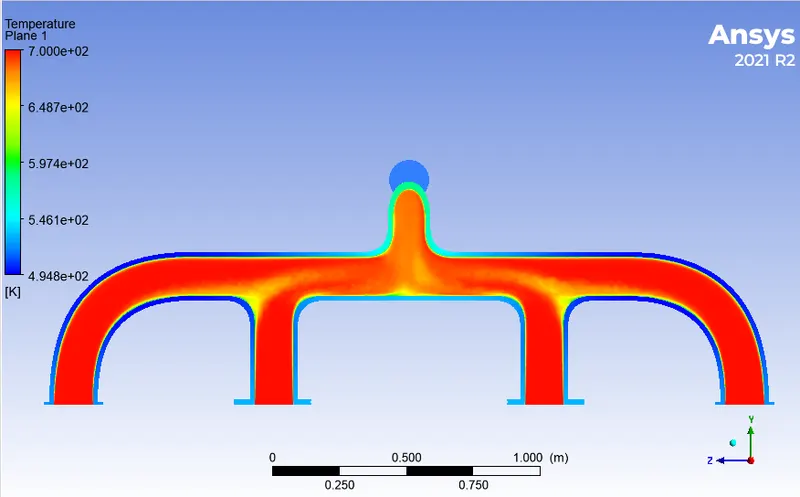
Temperature contour
pressure contour
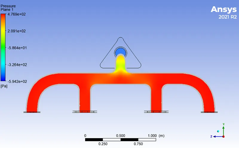
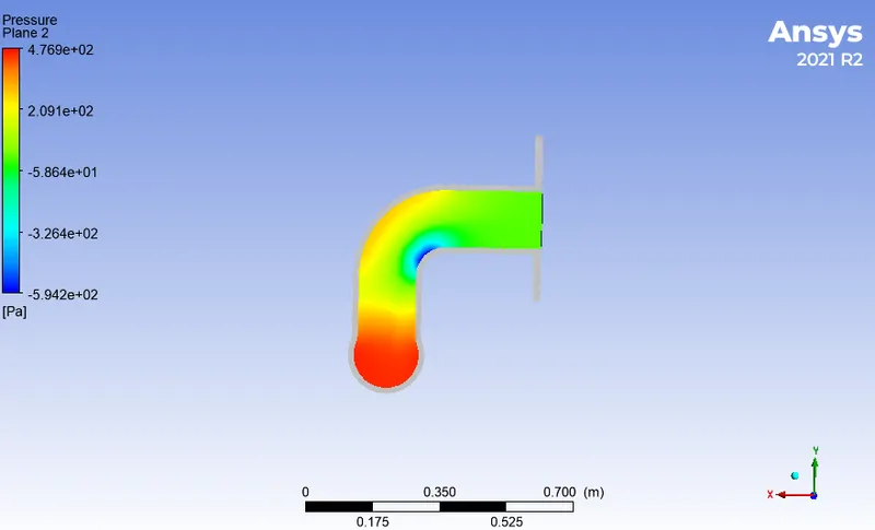
velocity contour
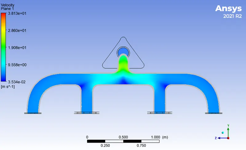
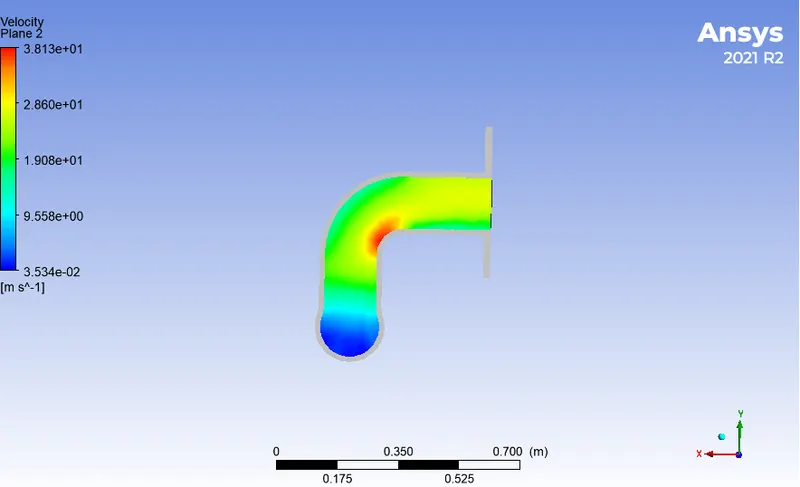
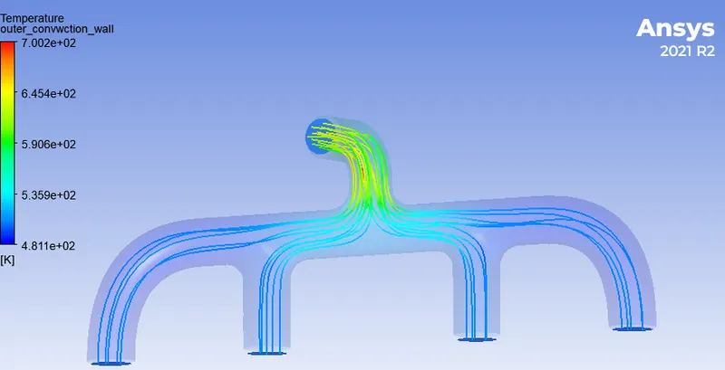
stream lines of velocity
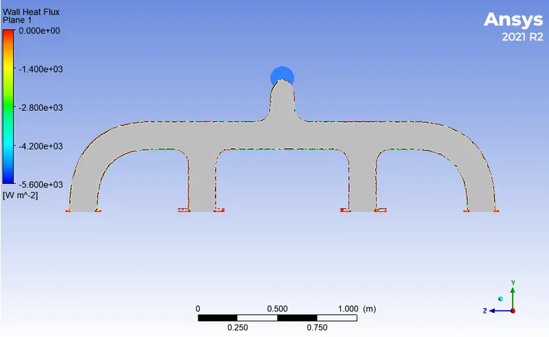
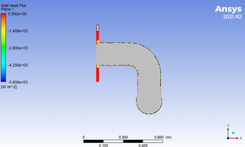
wall heat flux
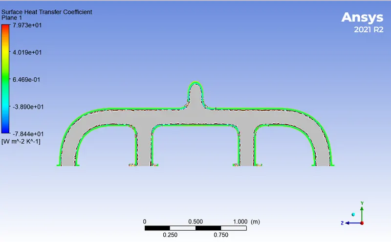
surface heat transfer coefficient
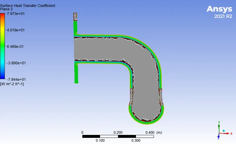
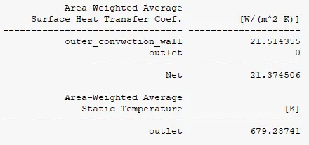
For Refined mesh results
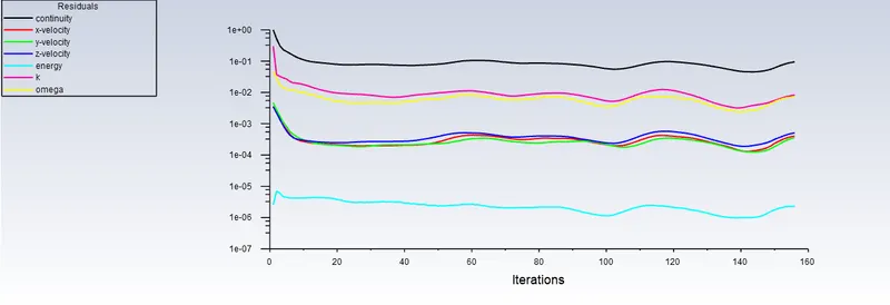
Scaled residuals
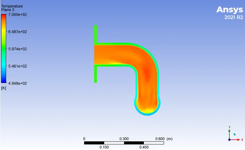
Temperature contour
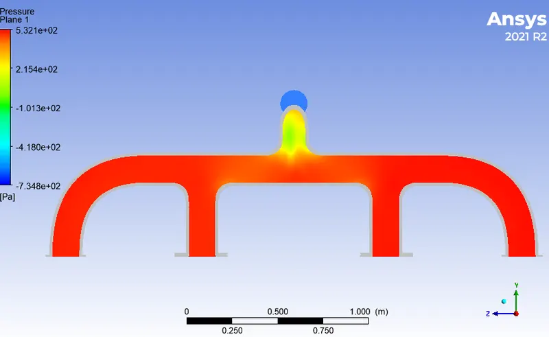
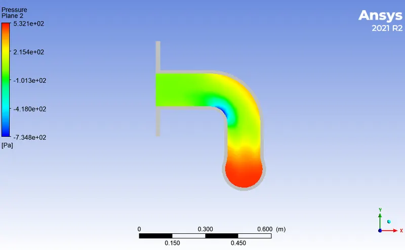
Pressure contour
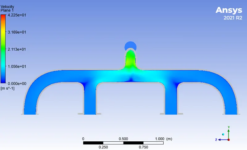
Velocity contour
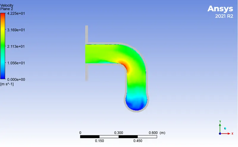
Streamlines of velocity
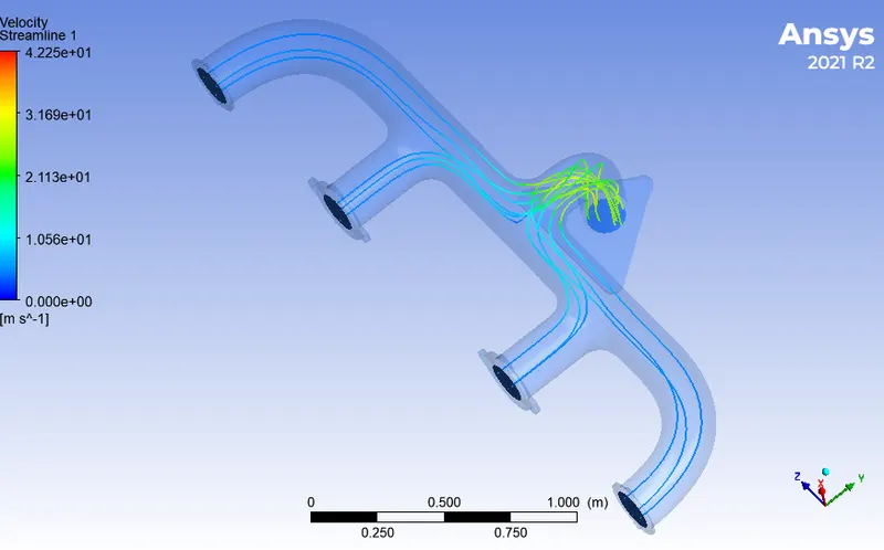
wall heat flux
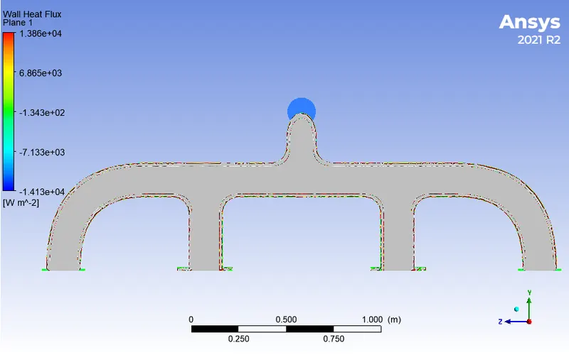
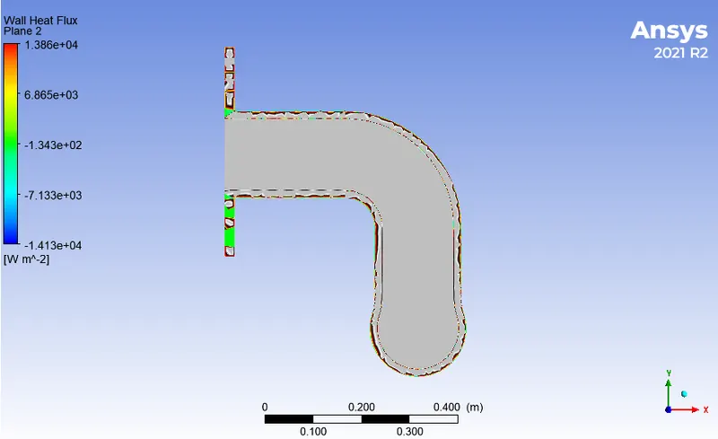
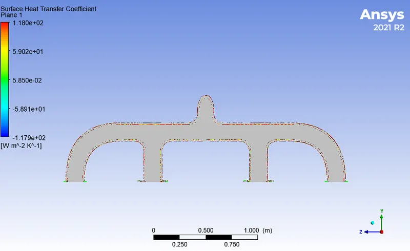
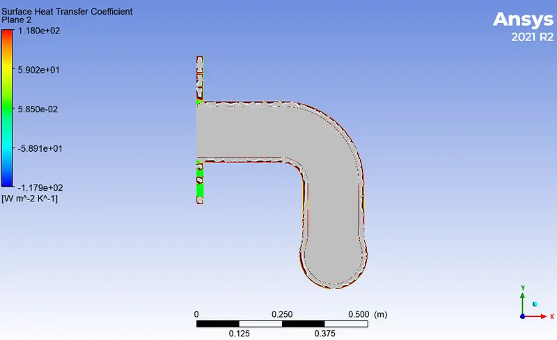
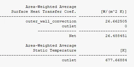
surface heat transfer coefficient
Output table
|
|
Element size (mm) |
No. of elements |
Surface Heat transfer coeff.`(W/m^2*k)` |
Outlet temperature (K) |
|
Baseline mesh |
150 |
134804 |
21.5 |
679 |
|
Refined mesh |
50 |
305910 |
26.6 |
677 |
Verify heat transfer coefficient
Under forced convection circumstances, we can determine the heat transfer coefficient by using the Dittus-Boelter correlation. Using the Dittus-Boelter correlation, the heat transfer coefficient can be calculated in the following way using two further dimensionless groups, the Reynolds number and the Prandtl number.
`h=(k/D_h )*Nu`
where k is the thermal conductivity of the liquid, `D_h` is the hydraulic diameter, and Nu is the Nusselt number which is determined by the following equation:
`Nu=0.023Re^0.8 Pr^n`
Where, n = 0.4 when fluid is being heated
N = 0.3 when fluid is being cooled
In this equation, Re is the Reynolds number which equates to:
`Re=(ρ*v*D)/μ=(1.225xx5xx0.1661)/1.7892`
And Pr is the Prandtl number:
`Pr=(C_p* μ)/k=(1006.43xx1.7892xx10^(-5))/0.0242,`
where `C_p` is heat capacity `Nu=0.023xx((1.225xx5xx0.1661)/1.7892)^0.8xx((1006.43xx1.7892xx10^(-5))/0.0242)^0.3=133.92`
Substituting the following value in the equation
`h=(Nu*k)/D=(133.92xx0.0242)/0.1661`
where, h = surface heat transfer coefficient
d = inner diameter
`h=19.5239W/(m^2 *k)`
- The value that has been obtained by this empirical relation is around the value that has been obtained by the simulation. This empirical relation is a primitive relation, and does not take into account the complexities of the pipe, or the various reasons of increased velocity and pressure drop but this equation gives us a value around which the value of the heat transfer coefficients should lie.
- Hence, we can say that the value obtained by the simulation is more or less accurate.
Conclusion
- From the above both cases we can observe that the refined mesh has more HTC value than baseline mesh.
- HTC increased in the refined mesh.