Conjugate Heat Transfer (CHT) Simulation through an Exhaust port of an In-line 4-Cylinder Engine

STEADY STATE CONJUGATE HEAT TRANSFER SIMULATION THROUGH AN EXHAUST PORT OF AN IN-LINE 4-CYLINDER ENGINE USING ANSYS FLUENT

1. AIM

Our aim is to simulate a steady state fluid flow through an exhaust port of an in-line 4-cylinder engine to study the conjugate heat transfer using ANSYS FLUENT.

2. THEORY/EQUATIONS/FORMULAE USED

ANSYS FLUENT academic version CFD package is used to carry out the simulation. It is a user friendly interface which provides high productivity and easy-to-use workflows. Workbench contains all workflow needed for solving a problem such as pre-processing, solving and post-processing.

Structure of ANSYS FLUENT simulations

The basic steps for a simulation are as follows,

1. Pre-processing – It includes geometry creation, discretization, providing named selection for using as boundary conditions. The packages used in pre-processing step are SpaceClaim, Ansys Mesher.
2. Solving – It includes applying initial and boundary conditions, adding material properties, applying suitable turbulence model as per the problem and running the iteration till convergence. The package used in post-processing step is Fluent.
3. Post-processing – It includes analyzing the results by plotting the results as charts, contour, and exporting the data, also validating the results both qualitatively and quantitatively. The package used in post-processing step is CFD-Post.

Conjugate Heat Transfer

Conjugate heat transfer is a combination of conduction and convection. It’s a heat transfer which involves the interaction of conduction within a solid body and convection between the solid surface and fluid volumes.

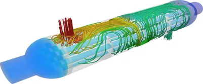
Typical example is a heat exchanger as in the figure the cold fluid enters the tubes and takes heat from the hot air flowing around the tube via natural convection. Some of the applications which involve conjugate heat transfers are building roofs, open water, chimney etc.

Heat Transfer Coefficient (HTC)

It’s a measure of convective heat transfer between fluid volume and solid medium around which the fluid flows.

Heat transfer coefficient is defined by the newton’s law of cooling. It is proportionality constant between heat flux (q) and temperature difference (ΔT) between the solid medium and the surrounding fluid. The SI unit of heat transfer coefficient (HTC) is watts per square meter kelvin (W/m²K).

For convective heat transfer coefficient calculation, usually T₂ is temperature of the solid surface and T₁ is temperature of the fluid around the surface or we can also call it as reference temperature. The choice of reference/ fluid temperature is important as the temperature near and away from the wall would be different depending on the flow due to thermal boundary layer.

There are two heat transfer coefficient for a flow through a pipe i.e. Internal HTC and External HTC

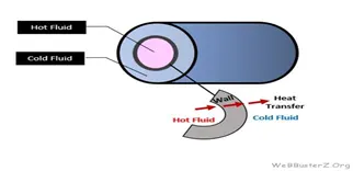
For External flows, fluid temperature will be the free stream temperature.

For Internal flow, fluid temperature will be the mass flow average temperature as the temperature profile inside a tube will be parabolic.

Nusselt Number

It is the ratio of convective heat transfer to the fluid heat conduction heat transfer under the same conditions.

Nu = q_convection /q_conduction

Convective heat transfer, q_convection = h*ΔT,

where h = Convective heat transfer coefficient, ΔT = Temperature difference

Conductive heat transfer, q_conduction = (k*ΔT)/ L,

where k = Thermal Conductivity of the fluid, ΔT = Temperature difference, L = characteristic length.

So, Nusselt Number, Nu = (h*L)/ k

Nusselt Number is also a function of Reynolds number and Prandtl number.

Dittus-Boelter equation – It’s an equation to calculate the Nusselt number for internal turbulent flow.

Exhaust Port - In-line 4 Cylinder Engine

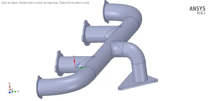
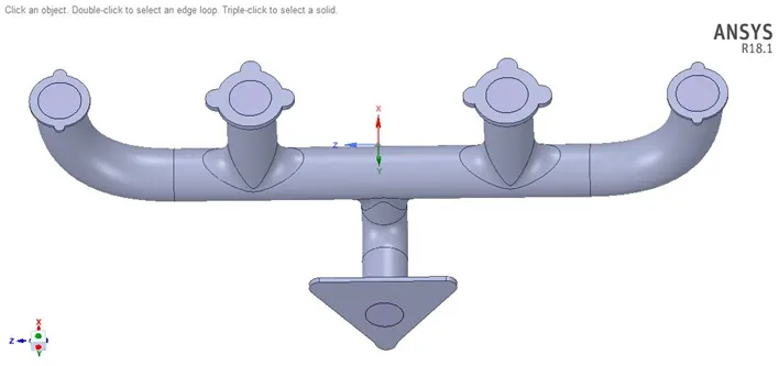
Fig: Different views for Exhaust Port

Problem – Flow via Exhaust Port

Steady state internal flow simulation through an exhaust port to study the conjugate heat transfer for a flow velocity of 5 m/s

Calculation

Reference values – Exhaust Port with 4 Inlets and 1 Outlet

Cylinder Port Dia = 200 mm

Steady State Internal Flow Simulation

Fluid chosen for the problem – Air, Inlet Temperature – 700 K, Internal ref. temperature – 300 K (Chosen)

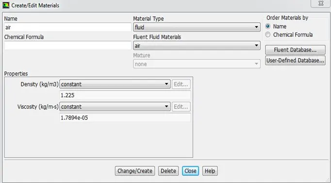
Density of Air = 1.225 kg/m3, Dynamic viscosity = 1.7894e-5 kg/ms, Velocity of fluid = 5 m/s,

So, Reynolds Number, Re = 68458.70

As the following analysis is done using two turbulence models i.e. k-omega & k-epsilon, the corresponding Y+ values are chosen.

Calculation of first cell height

For Y⁺ = 5 (For viscous sub layer, turbulence model = k-omega)

For Y⁺ = 50 (For turbulence layer, turbulence model = k-epsilon)

Skin Friction Coefficient, C_f

C_f = 0.058 * Re^(-0.2) [External Flow]

C_f = 0.079 * Re^(-0.25) [Internal Flow]

So, C_f = 0.00488 [using Internal Flow Eq.]

Wall Shear Stress, τ_w

τ_w = 0.5C_f ρu²

τ_w = 0.0747 N/m²

Frictional Velocity, U_t

U_t = (τ_w / ρ)^(1/2)

U_t = 0.25 m/s

Cell Height, y

y = Y⁺ * ν

U_t

where y = 0.30 mm (for Y⁺ = 5) and y = 2.92 mm (for Y⁺ = 50)

Total Thickness Calculation for Inflation layers

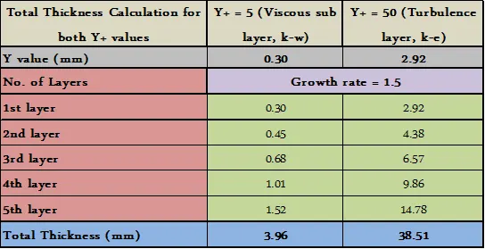
We can see from the above table the total thickness value with the growth rate of 1.5 for both the Y+ values are well within the range, Hence can be used for the simulation.

Inputs

External HTC – 20 W/m²k,

External Reference temperature – 300 K,

Inlet Temperature – 700 K,

Internal Reference temperature – 300 K

Output – Internal HTC - ??

Dittus-Boelter equation can be used to find the Nusselt number for internal turbulent pipe flow.

where Re – Reynolds number, Pr – Prandtl Number, D – Inside diameter of the circular duct, n – 0.3(fluid being cooled) / 0.4 (fluid being heated)

By using Pr – 0.71 for air at 700 K , Re_D = 68458.70, n = 0.4

Nu_D = 148.11

Calculate Heat Transfer Coefficient from Nusselt number formula

h = (Nu*k)/L

So, Internal HTC, h = 17.92 W/m²k

3. PROCEDURE

• In the process, firstly the geometry is imported in SpaceClaim and suitable clean up procedures are followed.
• Suitable geometry clean-up for 3-D exhaust port are such as deleting the duplicate edges, creating fluid volume by volume extract option, making both solid and fluid volume into single component and then sharing their topology by share prep to create a single interface for convection heat transfer between fluid and solid, and finally deleting the empty components.
• Baseline meshing is done to understand the problem and then to know how much and where the refinement is required in order to study the flow and all the boundaries are named respectively. Also checked the mesh quality is good enough to carry out the simulation.
• Material, solver type, the initial and boundary condition, suitable turbulence model are defined as per the problem. In the current problem 4 cases are defined with changes in turbulence model and the number of elements.
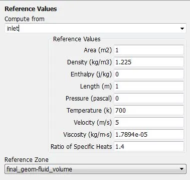
• In Ansys, for solving HTC of convection, heat flux needs to be defined. For external atmosphere we define both HTC and external ambient temperature and for internal atmosphere, internal reference temperature is defined in reference values option and the inlet temperature of the fluid entering is defined.
• So here we are defining external HTC and the internal, external temperatures are inputs and internal HTC is the output we are looking for.
• There are 2 ways to define the internal reference temperature based on the turbulence model we use. One is k-epsilon where the T_ref value is automatically taken from the centroid of the first cell and the second is the user input.
• The Y+ values are defined based on the turbulence model used. So for k-epsilon the Y+ 30 and for k-omega the Y+
• For k-e case the wall HTC is checked and for k-w case the surface HTC needs to be checked. So for surface HTC the solution data is exported in .cdat format and used in CFD post.
• The temperature contour on the outer wall convection, report definition for the average HTC is initiated in order to validate the essential features. Finally the animation is also added to study the overall behavior after the simulation is converged.

4. NUMERICAL ANALYSIS (Software used – ANSYS 2018 R1)

4.1 Geometric Model

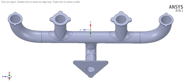
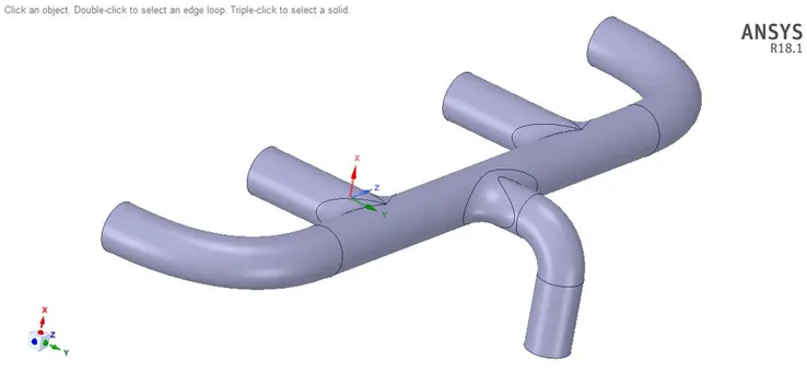
The 3D geometry of Exhaust Port is imported in SpaceClaim and the cleanup is done as per the figure given below.

3D Geometry with the flow domain – Ahmed Body

4.2 Mesh

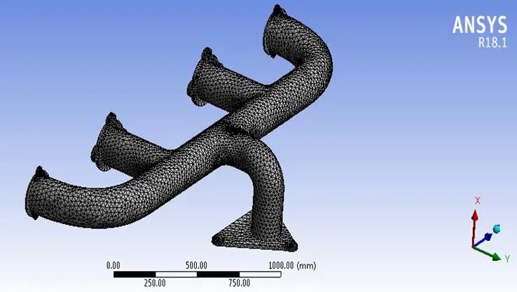
Fig: Baseline Mesh

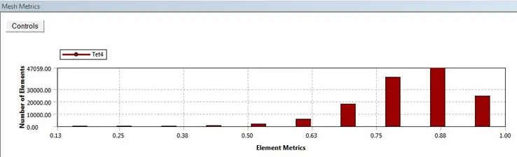
Fig: Element Quality

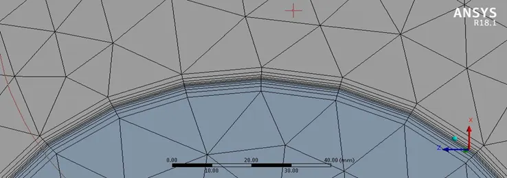
Fig: Inflation Layers

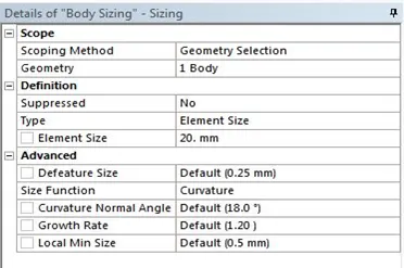
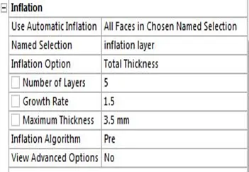
Fig: Size Function and Inflation Layer

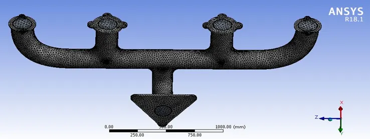
Fig: Final Mesh for the complete domain

4.3 Boundaries

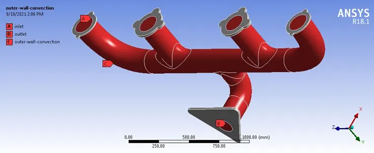
Fig: Boundaries for the complete domain

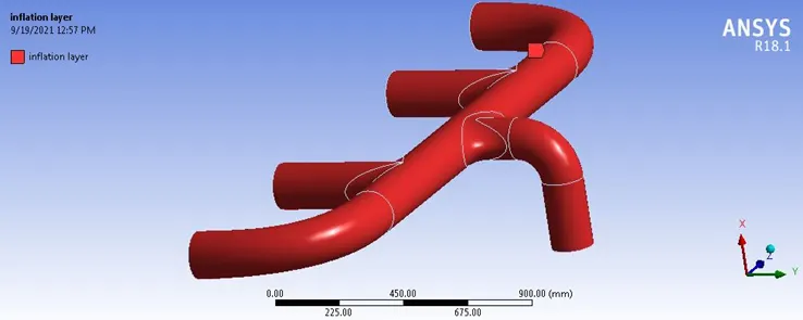
Fig: Inflation Layer Boundary

4.4 Solver Set-up

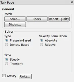
1. The mesh file is imported into the FLUENT software for the analysis of the modeled surface.
2. Once the mesh file is loaded and displayed, it is checked for the units, scale, and mesh.
3. There are two types of numerical solver methods pressure –based and density-based solver. The pressure based solver was used rather than the density based solver as the simulation is for lower Mach number. Absolute velocity formulation, steady state was used for the analysis.

4. Energy equation was switched on for the analysis process as we are interested in temperature of the system.

5. k-epsilon and k-omega turbulence models were used for the analysis as the Reynolds number used for simulation is in the range of 68458.70

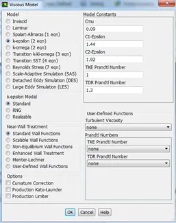
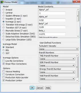
6. The fluid material chosen is air.

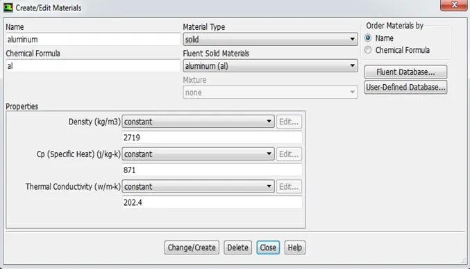
7. The surface of the solid volume is chosen as Aluminum.

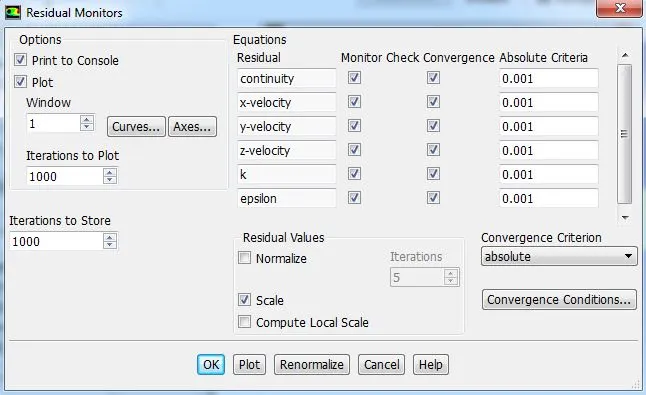
8. Convergence and monitor are checked for absolute criteria of 0.001 for all the residuals.

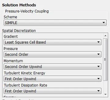
9. Solution methods – SIMPLE Scheme used for Pressure-Velocity coupling and the methods for Spatial Discretization are as per the below image.

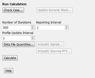
10. Hybrid initialization is done and numbers of iterations are set for running the steady simulation.

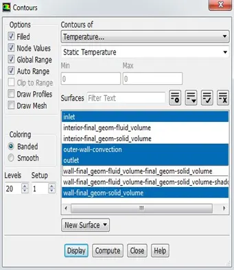
11. Temperature contours are set in order to monitor the variation during run time and also animations are added.

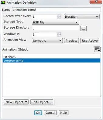
12. Reference Values are set to 700 K and 300 K for k-epsilon and k-omega turbulence model respectively.

Initial Setup and Boundary Condition

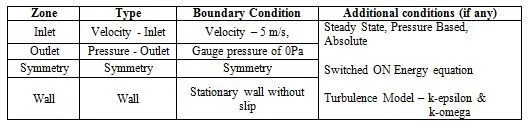
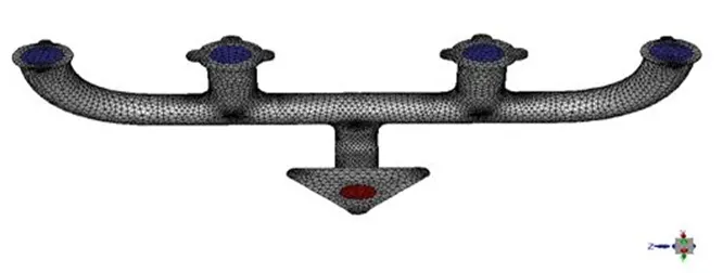
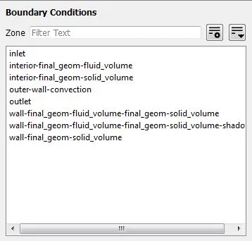
Fig. Boundaries

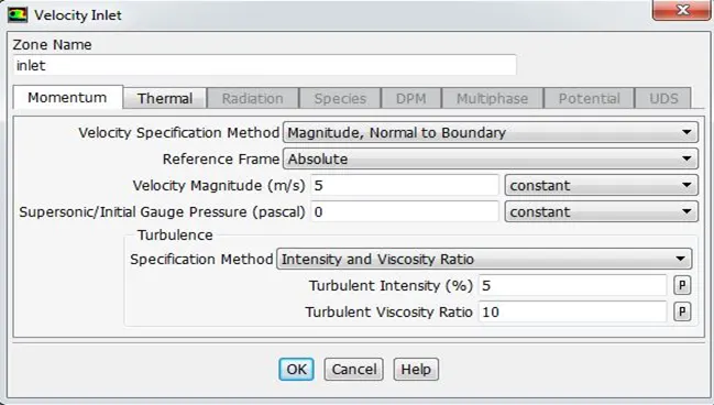
Fig. Inlet Boundary - Velocity

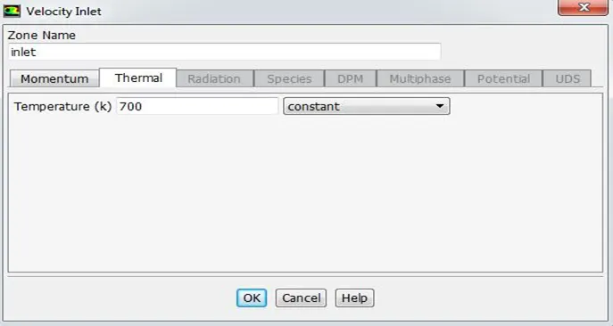
Fig. Inlet Boundary – Temperature

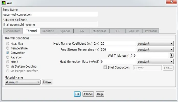
Fig. Wall Boundary – Thermal conditions – Convection

5. RESULTS

• Convergence Plot

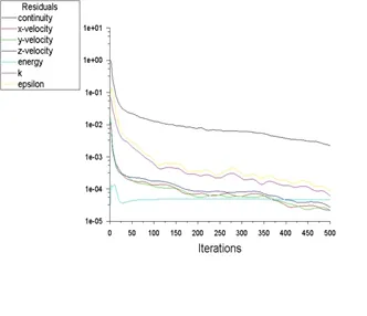
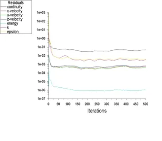
Fig: Case 1 Fig: Case 2

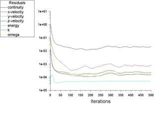
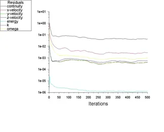
Fig: Case 3 Fig: Case 4

Video Link (Exhaust Port Simulation to study Conjugate Heat Transfer) - https://youtu.be/PUWEoNpmpx4

• Temp Contour on Outer Wall Convection

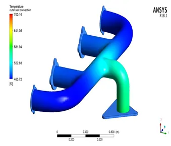
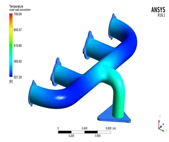
Fig: Case 1 Fig: Case 2

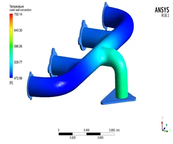
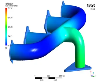
Fig: Case 3 Fig: Case 4

• Temp Contour at Inlet of the fluid Volume

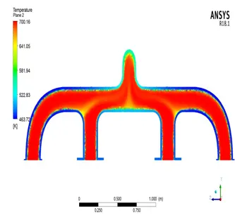
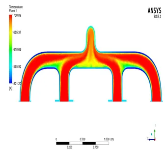
Fig: Case 1 Fig: Case 2

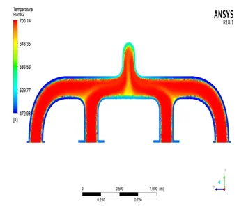
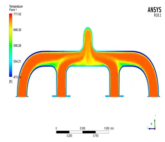
Fig: Case 3 Fig: Case 4

• Temp Contour at Outlet of the fluid Volume

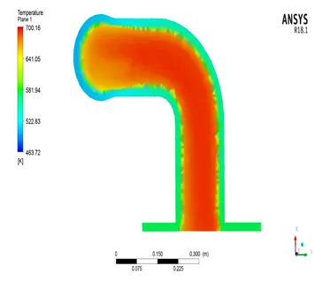
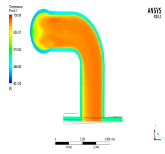
Fig: Case 1 Fig: Case 2

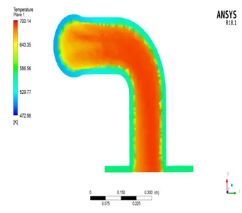
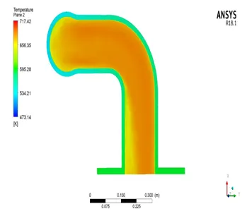
Fig: Case 3 Fig: Case 4

• Velocity contour at Inlet of the fluid Volume

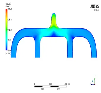
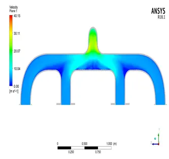
Fig: Case 1 Fig: Case 2

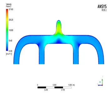
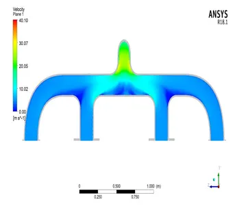
Fig: Case 3 Fig: Case 4

• Velocity contour at Outlet of the fluid Volume

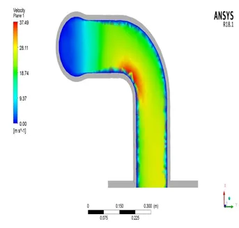
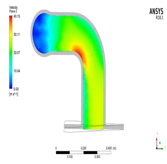
Fig: Case 1 Fig: Case 2

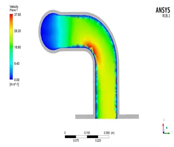
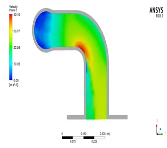
Fig: Case 3 Fig: Case 4

• Streamline Velocity Plot of flow in an Exhaust Port

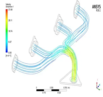
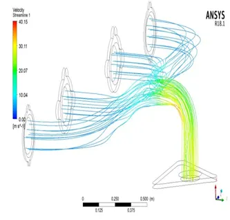
Fig: Case 1 Fig: Case 2

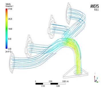
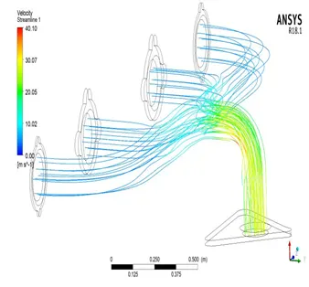
Fig: Case 3 Fig: Case 4

• Wall Heat Transfer Plot

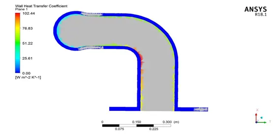
Fig: Case 1

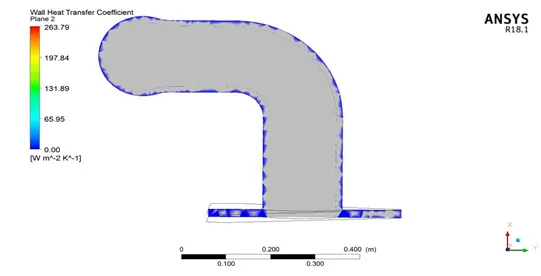
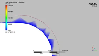
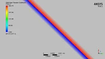
Fig: Case 2

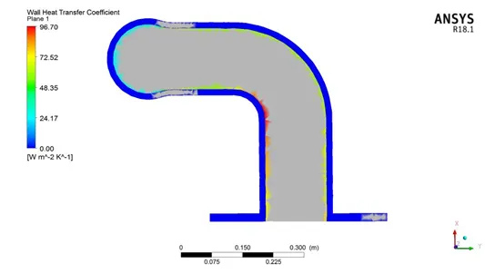
Fig: Case 3

• Surface Heat Transfer Plot on the Inflation Layer

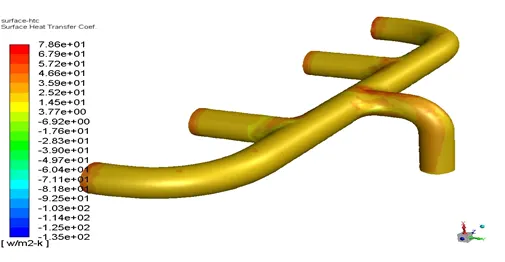
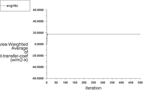
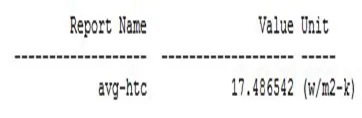
Fig: Case 4

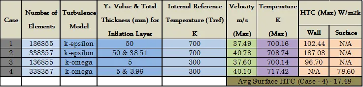
Comparison Study of all Cases

6. CONCLUSION

1. The steady state flow simulation through an Exhaust Port is done for flow velocity of 5 m/s in ANSYS FLUENT, from the convergence plot we can see that the solution remained more or less constant after 150 iterations although they didn’t get converged at least till 500 in all cases.
2. From the above comparison table, we can see and compare the values of velocity, temperature, HTC on the outer wall convection layer and inflation layer surface for different cases with different element sizes.
3. Firstly, it can be easily noticed that the values of maximum velocity, temperature, HTC for baselines mesh and refined mesh is almost similar and the variation in turbulence model doesn’t make any huge difference in this problem. But the contours of velocity and temperature obtained from the coarse mesh shows that, it is difficult to capture it clearly.
4. Wall HTC and Surface HTC is captured from outer wall convection boundary and inflation layer boundary respectively by maintaining the appropriate Y+ value for the turbulence model used.
5. The Temperature contour shows that the temperature increases when the flow from 4 different inlets combines and proceeds towards the outlet.
6. Velocity and HTC contours clearly shows that maximum heat transfer occurs at a location i.e. at the elbow where the velocity is more. Also in the validation perspective the simulation result of internal surface HTC from the simulaion and by mathematical calculation are similar in the same range (17.48-17.92). Hence the results are in good agreement and the underlying physics is visible clearly.
7. The acuracy of the prediction depends on the various factors such as the type of mesh (coarse/ fine), appropriate Y+ value of inflation layers for the turbulence model used, appropriate contours being analysed such as wall HTC for k-epsilon model and Surface HTC for k-omega model, proper reference temperature input.

7. REFERENCES

1. https://www.computationalfluiddynamics.com.au/tips-tricks-inflation-layer-meshing-in-ansys/
2. https://www.sciencedirect.com/science/article/abs/pii/S0017931006004455#:~:text=The%20term%20'conjugate%20heat%20transfer,moving%20over%20the%20solid%20surface.
3. https://www.simscale.com/docs/analysis-types/conjugate-heat-transfer-analysis/
4. https://www.researchgate.net/post/what_is_difference_between_surface_heat_transfer_coefficient_and_wallfunction_heat_transfer_coefficient
5. http://www.webbusterz.org/wp-content/uploads/2018/01/heat_transfer_through_a_pipe_wall-1.jpg
6. https://www.youtube.com/watch?v=fJDYtEGMgzs&ab_channel=FluidMechanics101
7. https://www.youtube.com/watch?v=ygR31_vhvJI&t=524s&ab_channel=FluidMechanics101
8. https://www.youtube.com/watch?v=PuTl98d0iZ0&t=1210s&ab_channel=FluidMechanics101
9. https://skill-lync.com/knowledgebase/convective-external-forced-heat-transfer-validation-2
10. https://skill-lync.com/knowledgebase/nusselt-number-2
11. https://en.wikipedia.org/wiki/Heat_transfer_coefficient