Numerical Simulation of Quasi 1D Super-sonic C-D nozzle flow using Mac-Cormack Method

NUMERICAL SIMULATION OF QUASI 1D SUPERSONIC C-D NOZZLE FLOW USING MAC-CORMACK METHOD

1. AIM

Our aim is to write a program to solve the governing flow equations to simulate the quasi 1D supersonic Convergent-Divergent nozzle flow using Mac-Cormack method.

2. THEORY/EQUATIONS/FORMULAE USED

Flow Governing Equations include continuity, momentum and energy equation. The equations are modified as per the problem and purpose to solve.

Variables in the governing equations are converted non-dimensional for the convenience of calculation, but there is no real difference between dimensional and non-dimensional terms. In this problem, two different forms of governing equation are solved using Mac-Cormack method.

Mac-Cormack method – It is a numerical discretization technique where equations are solved explicitly in the time marching approach. The time marching approach is divided in two phases such as predictor and corrector step. In the predictor and corrector step process, forward and rearward difference schemes are used respectively for space terms.

Then the initial and boundary conditions are applied to calculate the primitive variables such as Density, Temperature, Pressure, Mach number and Mass flow rate using the equations.

The two forms of flow governing equations used are Non-Conservative and Conservative.

Governing Flow Equations,

1. Non-Conservative form – Control volume (CV) is moving, so the fluid element inside the CV remains same.

2. Conservative form - Control volume (CV) is stationery, so the fluid element inside the CV keeps changing.

Continuity: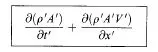

Momentum: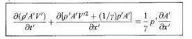

Energy:

The governing equations in conservative form can be represented in a generic form as shown below which consists of solution vectors U, flux vectors F, and source term J such as given below,

where U₁ = ρ’ A’

U₂ = ρ’ A’V’

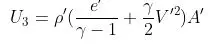
F₁ = ρ’ A’V’

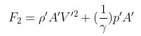
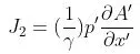
In conservative form, the primitive variables cannot be calculated directly as it represented in the generic form. So the solution vectors, flux vectors, and source term variables are calculated using Mac-Cormack method and then primitive variables need to be extracted from it.

Mesh - 1D Grids along the C-D Nozzle

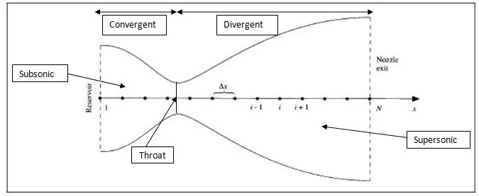
Given inputs

Nozzle Area, A = 1+ 2.2(x-1.5)², 0 ≤ x ≤ 3

Non-Conservative form

a) Initial Condition at t = 0

Density, ρ = 1 – 0.3146x,

Temperature, T = 1 – 0.2314x,

Velocity, V = (0.1+1.09x)T^1/2

b) Boundary Condition

Inflow, V₁ = 2 V_{2 –} V₃

Outflow, V₃₁ = 2 V_{30 –} V₂₉ Mach number, M = V/ sqrt.(T)

ρ ₃₁ = 2 ρ _{30 –} ρ ₂₉

T ₃₁ = 2 T _{30 –} T ₂₉

Conservative form

a) Initial Condition

ρ' = 1, T’ = 1} for 0 ≤ x’≤ 0.5

ρ' = 1-0.366(x’-0.5), T’ = 1-0.167(x’-0.5)} for 0.5 ≤ x’≤ 1.5

ρ' = 0.634-0.3879(x’-0.5), T’ = 0.833-0.3507(x’-0.5)} for 1.5 ≤ x’≤ 3.0

b) Boundary Condition

Inflow, U_{1 (i=1)} = (ρ’ A’) _i=1 ρ’ & T’ = 1, So U₁ = A’_(i=1)

U_{2 (i=1)} = 2 U_{2 (i=2) –} U_{2 (i=3)}

Outflow, (U₁) _N = 2 (U₁) _N–1 - (U₁) _N-2 Mach number, M = V/ sqrt.(T)

(U₂) _N = 2 (U₂) _N–1 - (U₂) _N-2

(U₃) _N = 2 (U₃) _N–1 - (U₃) _N-2

3. OBJECTIVES & PROCEDURE

• The main objective of the challenge is to write code to solve the two different forms i.e, Conservative and Non-Conservative form of governing equations using Mac-Cormack method and understand the difference based on the results.
• In the process, firstly both forms of governing equations are turned non-dimensional. 1D grid is set along the nozzle x-axis alone as we consider it as quasi 1D supersonic CD nozzle.
• Both the forms of governing equations are discretized using Mac-Cormack method. Initial and Boundary condition are applied as given in the problem.
• The primitive variables such as Density, Temperature, Pressure, Mach number and Mass flow rate are calculated using the equations.
• All the results are plotted in graph.

4. PROGRAM

Programming language used – Octave 5.1.1

Main Program
-----------------------------------------------------------------------------------------
clear all
close all
clc

% 1D Quasi Steady Supersonic Nozzle Flow using Mac-Cormack Method
% Non-Conservative approach Vs Conservative approach

% Inputs
n = 31;
x = linspace(0,3,n);
dx = x(2)-x(1);

% Constants
throat = (n+1)/2;
gamma = 1.4;

% Number of Time steps
nt = 1400;

% Initial Profiles
% Area
A = 1+(2.2*((x-1.5).^2));
dA = A(15)-A(16);

% Density
rho = 1-(0.3146*x);

for i = 1:n 

  if (x(i)>=0) & (x(i)<=0.5)
    rho_c(i) = 1;
    T_c(i) = 1;
    
  elseif (x(i)>0.5) & (x(i)<=1.5)
    rho_c(i) = 1-(0.366.*(x(i)-0.5));
    T_c(i) = 1-(0.167.*(x(i)-0.5));
  
  else (x(i)>1.5) &(x(i)<=3)
    rho_c(i) = 0.634-(0.3879.*(x(i)-1.5));
    T_c(i) = 0.833-(0.3507.*(x(i)-1.5));
    
  end  
  V_c(i) = (0.59)./(rho_c(i).*A(i));
end
% Temperature
T = 1-(0.2314*x);

% Velocity
V = (0.1+(1.09*x)).*T.^0.5; 

C = 0.5;

% Time step
dt = min(C.*(dx./(sqrt(T)+V)))
dt_c = min(C.*(dx./(sqrt(T_c) + V_c)))

% Solution vectors of conservation form
U_1 = rho_c.*A;
U_2 = rho_c.*A.*V_c;
U_3 = rho_c.*((T_c./(gamma - 1))+(gamma*0.5.*(V_c.^2))).*A;

for i = 1:n
rho_e(i) = 0.634;
T_e(i) = 0.833;
P_e(i) = rho_e(i)*T_e(i);
M_e(i) = 1;
m_exact(i) = rho_e(i)*sqrt(T_e(i));
end
% Non_conservative_form
tic
[rho rho_t T T_t P P_t M M_t m] = Non_conservative_form(n,x,dx,A,rho,T,V,throat,gamma,nt,dt);
non_conservative_form_time = toc

% Plotting
% Flow field variables
% Density
  figure(1)
  subplot(4,1,1)
  plot(x,rho,'Linewidth',2)
  ylabel('Density')
  legend('Non-Conservative Form')
  title('Steady state distribution of flow field variables Vs nozzle length','Fontsize',14)
 
% Pressure ratio
  subplot(4,1,2)
  plot(x,P,'Linewidth',2)
  ylabel('Pressure')
    
% Temperature
  subplot(4,1,3)
  plot(x,T,'Linewidth',2)
  ylabel('Temperature')
    
% Mach Number
  subplot(4,1,4)
  plot(x,M,'Linewidth',2)
  xlabel('Nozzle Length')
  ylabel('Mach Number')

% Timewise variations of Flow field variables at Nozzle throat  
% Density
  figure(2)
  subplot(4,1,1)
  plot(1:nt,rho_t,'r','Linewidth',2)
  ylabel('Density')
  legend('Non-Conservative Form')
  title('Time wise variation of flow field variables @ nozzle throat','Fontsize',14)
 
% Pressure ratio
  subplot(4,1,2)
  plot(1:nt,P_t,'r','Linewidth',2)
  ylabel('Pressure')
   
% Temperature
  subplot(4,1,3)
  plot(1:nt,T_t,'r','Linewidth',2)
  ylabel('Temperature')
    
% Mach Number
  subplot(4,1,4)
  plot(1:nt,M_t,'r','Linewidth',2)
  xlabel('Number of Iterations')
  ylabel('Mach Number')
  
% Conservative_form
tic
[rho_c rho_tc T_c T_tc P_c P_tc V_c M_c M_tc m_c U_1 U_2 U_3] = Conservative_form(n,x,dx,A,dA,rho_c,V_c,T_c,U_1,U_2,U_3,throat,gamma,nt,dt_c);
conservative_form_time = toc

##[x' A' rho_c' V_c' T_c' P_c' M_c' m_c' U_1' U_2' U_3']
 
 
% Plotting
% Flow field variables
% Density
  figure(4)
  subplot(4,1,1)
  plot(x,rho_c,'Linewidth',2)
  ylabel('Density')
  legend('Conservative Form')
  title('Steady state distribution of flow field variables Vs nozzle length','Fontsize',14)
 
% Pressure ratio
  subplot(4,1,2)
  plot(x,P_c,'Linewidth',2)
  ylabel('Pressure')
    
% Temperature
  subplot(4,1,3)
  plot(x,T_c,'Linewidth',2)
  ylabel('Temperature')
    
% Mach Number
  subplot(4,1,4)
  plot(x,M_c,'Linewidth',2)
  xlabel('Nozzle Length')
  ylabel('Mach Number')

% Timewise variations of Flow field variables at Nozzle throat  
% Density
  figure(5)
  subplot(4,1,1)
  plot(1:nt,rho_tc,'r','Linewidth',2)
  ylabel('Density')
  legend('Conservative Form')
  title('Time wise variation of flow field variables @ nozzle throat','Fontsize',14)
 
% Pressure ratio
  subplot(4,1,2)
  plot(1:nt,P_tc,'r','Linewidth',2)
  ylabel('Pressure')
   
% Temperature
  subplot(4,1,3)
  plot(1:nt,T_tc,'r','Linewidth',2)
  ylabel('Temperature')
    
% Mach Number
  subplot(4,1,4)
  plot(1:nt,M_tc,'r','Linewidth',2)
  xlabel('Number of Iterations')
  ylabel('Mach Number')

% Normalized mass flow rate distributions
  figure(7)
  plot(x,m,'Linewidth',2) 
  hold on
  plot(x,m_c,'Linewidth',2)
  hold on
  plot(x,m_exact,'Linewidth',2) 
  title('Normalized mass flow rate distributions of non conservative Vs conservative form equation','Fontsize',14)
  xlabel('Nozzle Length','Fontsize',14)
  ylabel('Mass Flow rate','Fontsize',14)
  legend('Non-Conservative Form','Conservative Form','Exact Value')
  
% Grid Independence Study
  Grid_Independence_Study =[rho_e(31) T_e(31) P_e(31) M_e(31);rho_t(1400) T_t(1400) P_t(1400) M_t(1400);rho_tc(1400) T_tc(1400) P_tc(1400) M_tc(1400)];
---------------------------------------------------------------------------------------

Function Program - Non-conservation form
---------------------------------------------------------------------------------------
function [rho rho_t T T_t P P_t M M_t m] = Non_conservative_form(n,x,dx,A,rho,T,V,throat,gamma,nt,dt)

%Outer time loop
 for k = 1:nt
  
  rho_old = rho;
  T_old = T;
  V_old = V;
  
  % Predictor Step
  for i = 2:n-1
    %Derivative terms
     dvdx(i) =(V(i+1)-V(i))/dx;
     dlogAdx(i) =(log(A(i+1))-log(A(i)))/dx;
     drhodx(i) =(rho(i+1)-rho(i))/dx;
     dtdx(i) = (T(i+1)-T(i))/dx;
     
     % Continuity equation 
     drho_dt_p(i) = -rho(i)*dvdx(i) -(rho(i)*V(i)*dlogAdx(i)) - (V(i)*drhodx(i));
     
     % Momentum equation
     dV_dt_p(i) = -V(i)*dvdx(i) - ((1/gamma)*(dtdx(i) + ((T(i)/rho(i))*drhodx(i))));
     
     % Energy equation
     dT_dt_p(i) = -V(i)*dtdx(i) - ((gamma - 1)*T(i)*(dvdx(i) + V(i)*dlogAdx(i)));
     
     % Updating values
     rho(i) = rho(i) + drho_dt_p(i)*dt;
     V(i) = V(i) + dV_dt_p(i)*dt;
     T(i) = T(i) + dT_dt_p(i)*dt;
  end    
  
  % Corrector Step
  for i = 2:n-1
    %Derivative terms
     dvdx(i) =(V(i)-V(i-1))/dx;
     dlogAdx(i) =(log(A(i))-log(A(i-1)))/dx;
     drhodx(i) =(rho(i)-rho(i-1))/dx;
     dtdx(i) = (T(i)-T(i-1))/dx;
     
     % Continuity equation 
     drho_dt_c(i) = -rho(i)*dvdx(i) -(rho(i)*V(i)*dlogAdx(i)) - (V(i)*drhodx(i));
     
     % Momentum equation
     dV_dt_c(i) = -V(i)*dvdx(i) - ((1/gamma)*(dtdx(i) + ((T(i)/rho(i))*drhodx(i))));
     
     % Energy equation
     dT_dt_c(i) = -V(i)*dtdx(i) - ((gamma - 1)*T(i)*(dvdx(i) + V(i)*dlogAdx(i)));
    
  end      
  % Calculating average values
  drho_dt_avg = 0.5*(drho_dt_p+drho_dt_c);
  dV_dt_avg = 0.5*(dV_dt_p+dV_dt_c);
  dT_dt_avg = 0.5*(dT_dt_p+dT_dt_c);
  
  for i = 2:n-1
    % Actual values for next time steps
    rho(i) = rho_old(i) + drho_dt_avg(i)*dt;
    V(i) = V_old(i) + dV_dt_avg(i)*dt;
    T(i) = T_old(i) + dT_dt_avg(i)*dt;
  end 
  % Boundary Conditions
  % Inlet
    V(1) = 2*V(2) - V(3);
  
  % Outlet
    rho(n) = 2*rho(n-1) - rho(n-2);
    V(n) = 2*V(n-1) - V(n-2);
    T(n) = 2*T(n-1) - T(n-2);
  
  for i = 1:n
    P(i) = rho(i)*T(i);
    M(i) = V(i)/sqrt(T(i));
    m(i) = rho(i)*A(i)*V(i); 
  end
   
  % Flow Field @ Nozzle Throat 
  rho_t(k) = rho(throat);
  T_t(k) = T(throat);
  P_t(k) = P(throat);
  M_t(k) = M(throat);
  
  % Non_dimensional_mass_flow
 if k == 50 
      figure(3)
      plot(x,m,'Linewidth',2)
      hold on
    elseif k == 100
      plot(x,m,'Linewidth',2)   
      hold on
    elseif k == 150
      plot(x,m,'Linewidth',2)     
      hold on
    elseif k == 200
      plot(x,m,'Linewidth',2)
      hold on
    elseif k == 700
      plot(x,m,'Linewidth',2)
      title('Variation of mass flow rate distribution inside the nozzle @ different time steps','Fontsize',14)
      xlabel('Nozzle Length','Fontsize',14)
      ylabel('Non dimensional mass flow','Fontsize',14)
      legend('50 dt','100 dt','150 dt','200 dt','700 dt')
 end     
 end  
end
---------------------------------------------------------------------------------------

Function Program - Conservation form
---------------------------------------------------------------------------------------
function [rho_c rho_tc T_c T_tc P_c P_tc V_c M_c M_tc m_c U_1 U_2 U_3] = Conservative_form(n,x,dx,A,dA,rho_c,V_c,T_c,U_1,U_2,U_3,throat,gamma,nt,dt_c)

%Outer time loop
 for k = 1:nt
    U_1_old = U_1;
    U_2_old = U_2;
    U_3_old = U_3;
  
    F_1 = U_2;
    F_2 = (U_2.^2./U_1)+(((gamma - 1)/gamma).*(U_3-(0.5*gamma*(U_2.^2./U_1))));
    F_3 = (gamma*((U_2.*U_3)./U_1))- (0.5*gamma*(gamma-1)*((U_2.^3)./(U_1.^2)));
     
  % Predictor Step
  for i = 2:n-1
     
     dA_dx_p(i) = (A(i+1)-A(i))/dx;
     
     J_2(i) = (1/gamma)*rho_c(i).*T_c(i)*(dA_dx_p(i));
    
    %Derivative terms
     dF_1_dx(i) =(F_1(i+1)-F_1(i))/dx;
     dF_2_dx(i) =(F_2(i+1)-F_2(i))/dx;
     dF_3_dx(i) =(F_3(i+1)-F_3(i))/dx;
         
     % Continuity equation 
     dU_1_dt_p(i) = -dF_1_dx(i);
     
     % Momentum equation
     dU_2_dt_p(i) = -dF_2_dx(i)+ J_2(i);
     
     % Energy equation
     dU_3_dt_p(i) = -dF_3_dx(i);
     
     % Updating values
     U_1(i) = U_1(i) + dU_1_dt_p(i)*dt_c;
     U_2(i) = U_2(i) + dU_2_dt_p(i)*dt_c;
     U_3(i) = U_3(i) + dU_3_dt_p(i)*dt_c;
  end     
  
  % Primitive variables from solution vectors  
    rho_c = U_1./A;
    V_c = U_2./U_1;
    T_c = (gamma - 1).*((U_3./U_1) - (0.5*gamma.*(U_2./U_1).^2));
  
  % Flux Vectors
    F_1 = U_2;
    F_2 = (U_2.^2./U_1)+(((gamma - 1)/gamma).*(U_3-(0.5*gamma.*((U_2.^2)./U_1))));
    F_3 = (gamma.*((U_2.*U_3)./U_1))- (0.5*gamma*(gamma-1).*((U_2.^3)./(U_1.^2)));
 
  % Corrector Step
  for i = 2:n-1
     dA_dx_c(i) = (A(i)-A(i-1))/dx;
     
     J_2(i) = (1/gamma)*rho_c(i)*T_c(i)*(dA_dx_c(i));
        
    %Derivative terms
     dF_1_dx(i) =(F_1(i)-F_1(i-1))/dx;
     dF_2_dx(i) =(F_2(i)-F_2(i-1))/dx;
     dF_3_dx(i) =(F_3(i)-F_3(i-1))/dx;
         
     % Continuity equation 
     dU_1_dt_c(i) = -(dF_1_dx(i));
     
     % Momentum equation
     dU_2_dt_c(i) = -dF_2_dx(i)+ J_2(i);
     
     % Energy equation
     dU_3_dt_c(i) = -(dF_3_dx(i));
    
  end      
  
  % Calculating average values
  dU_1_dt_avg = 0.5*(dU_1_dt_p+dU_1_dt_c);
  dU_2_dt_avg = 0.5*(dU_2_dt_p+dU_2_dt_c);
  dU_3_dt_avg = 0.5*(dU_3_dt_p+dU_3_dt_c);

  for i = 2:n-1
    % Actual values for next time steps
    U_1(i) = U_1_old(i) + dU_1_dt_avg(i)*dt_c;
    U_2(i) = U_2_old(i) + dU_2_dt_avg(i)*dt_c;
    U_3(i) = U_3_old(i) + dU_3_dt_avg(i)*dt_c;
  end 
  
  % Boundary Conditions
  % Inlet
    U_1(1) = rho_c(1).*A(1);
    U_2(1) = 2*U_2(2) - U_2(3);
    
    V_c(1) = U_2(1)./U_1(1);
    
    U_3(1) = U_1(1).*((T_c(1)/(gamma - 1))+(gamma*0.5.*(V_c(1).^2)));
    
  % Outlet
    U_1(n) = 2*U_1(n-1) - U_1(n-2);
    U_2(n) = 2*U_2(n-1) - U_2(n-2);
    U_3(n) = 2*U_3(n-1) - U_3(n-2);

 
  % Primitive variables from solution vectors 
    rho_c = U_1./A;
    V_c = U_2./U_1;
    T_c =(gamma - 1).*((U_3./U_1)-(0.5*gamma.*(U_2./U_1).^2)); 
 
  for i = 1:n
    P_c(i) = rho_c(i).*T_c(i);
    M_c(i) = V_c(i)./sqrt(T_c(i));
    m_c(i) = rho_c(i).*A(i).*V_c(i); 
  end
  
  % Flow Field @ Nozzle Throat 
    rho_tc(k) = rho_c(throat);
    T_tc(k) = T_c(throat);
    P_tc(k) = P_c(throat);
    M_tc(k) = M_c(throat);
  
  % Non_dimensional_mass_flow
 if k == 50 
      figure(6)
      plot(x,m_c,'Linewidth',2)
      hold on
    elseif k == 100
      plot(x,m_c,'Linewidth',2)   
      hold on
    elseif k == 150
      plot(x,m_c,'Linewidth',2)     
      hold on
    elseif k == 200
      plot(x,m_c,'Linewidth',2)
      hold on
    elseif k == 700
      plot(x,m_c,'Linewidth',2)
      title('Variation of mass flow rate distribution inside the nozzle @ different time steps','Fontsize',14)
      xlabel('Nozzle Length','Fontsize',14)
      ylabel('Non dimensional mass flow rate','Fontsize',14)
      legend('50 dt','100 dt','150 dt','200 dt','700 dt')
 end     
 end  
end
---------------------------------------------------------------------------------------

5. RESULTS

5.1 Non-Conservative V/s Conservative form (31 Grid points)

1. Steady-state distribution of primitive variables inside the nozzle

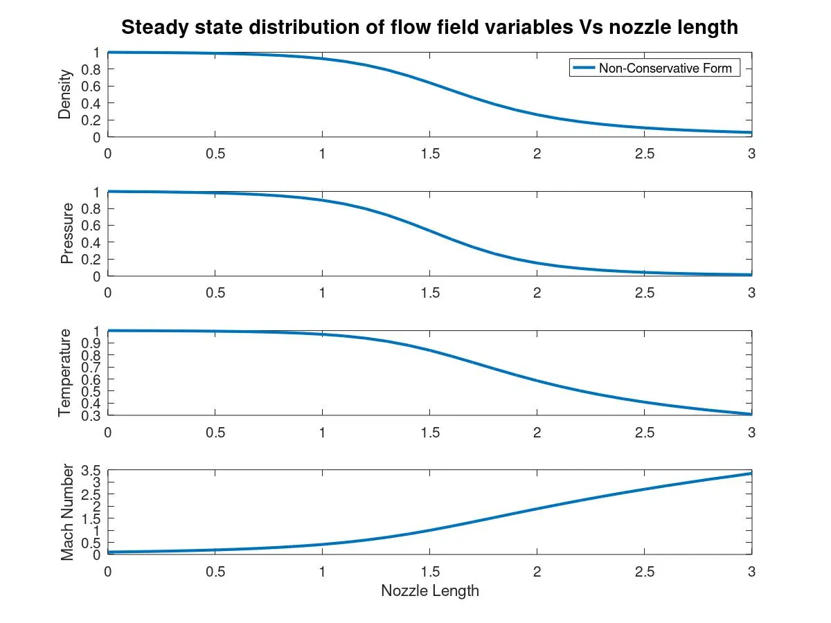
Graph 1

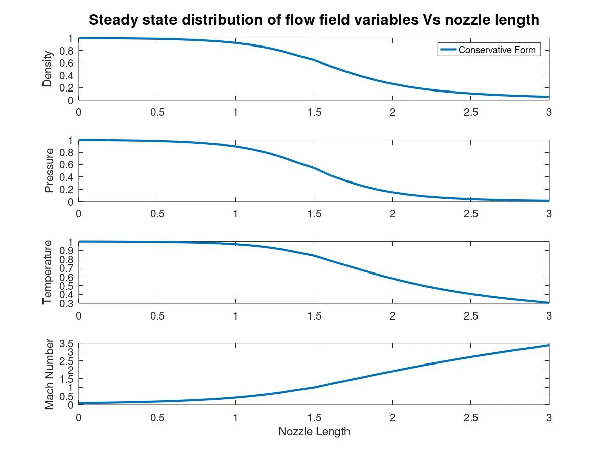
Graph 2

Graph 1 and 2 shows the flow field variables along the nozzle length in non-conservative and conservative form respectively. Primitive variales such as Density, Temperature and Pressure are high at the inlet and starts decresing after the throat section of the CD Nozzle whereas the Mach number is very low at the inlet but starts increasing and attains supersonic speed at the outlet. The behaviour of the curve of each variable is almost same in both forms.

2. Time-wise variation of the primitive variables

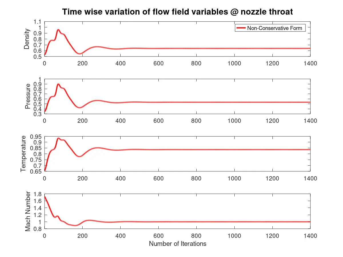
Graph 3

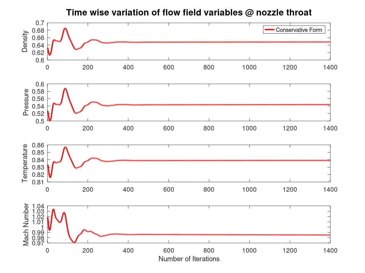
Graph 4

Graph 3 and 4 shows that the time wise variation variation of flow field variables such as Density, Temperature, Pressure and Mach number values at nozzle throat in non-conservative and conservative form respectively. The fluctuation of values is more at the beginning in conservative form than the non-conservative form. The values becomes constant only after around 300 iterations at throat section of CD nozzle (node, i=16) approximately in both forms.

3. Variation of Mass flow rate distribution inside the nozzle at different time steps

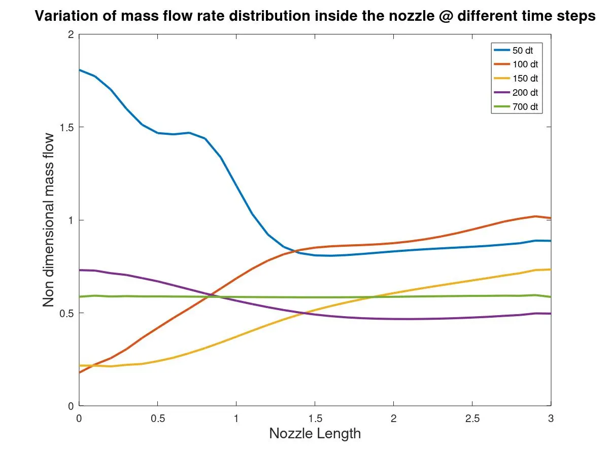
Graph 5

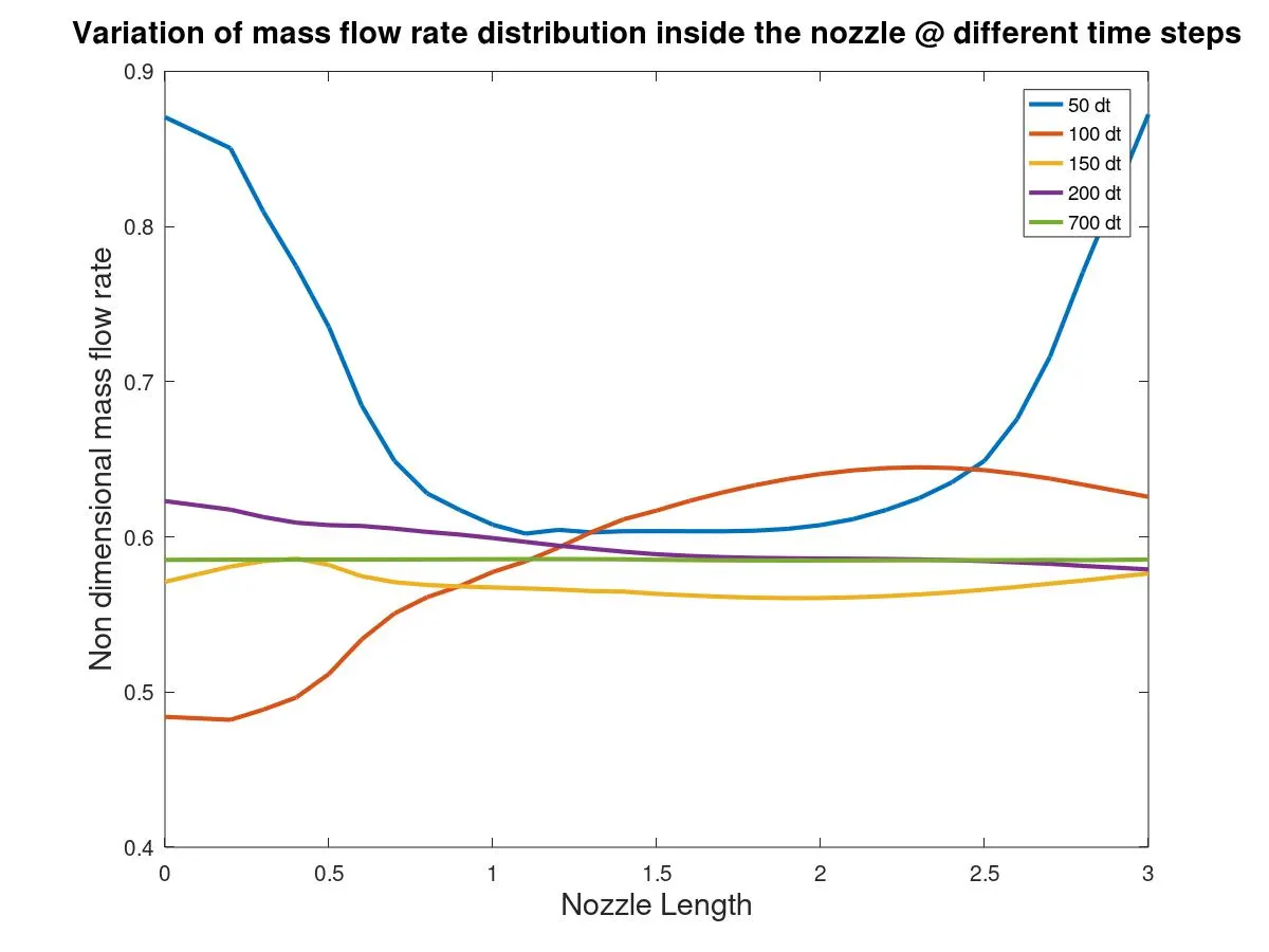
Graph 6

Graph 5 and 6 indicates the mass flow rate along the nozzle length at different time steps such as 50, 100, 150, 200 and 700 in non-conservative and conservative form respectively. We can observe that mass flow rate at 50 dt fluctuates a lot in the beginning and stabilizes after halfway through the nozzle length in non-conservative form but the values again shoots up at the outlet in conservative form. The exact mass flow rate values is achived only after 700 time steps in both forms.

4. Comparison of Normalized mass flow rate distributions of both forms

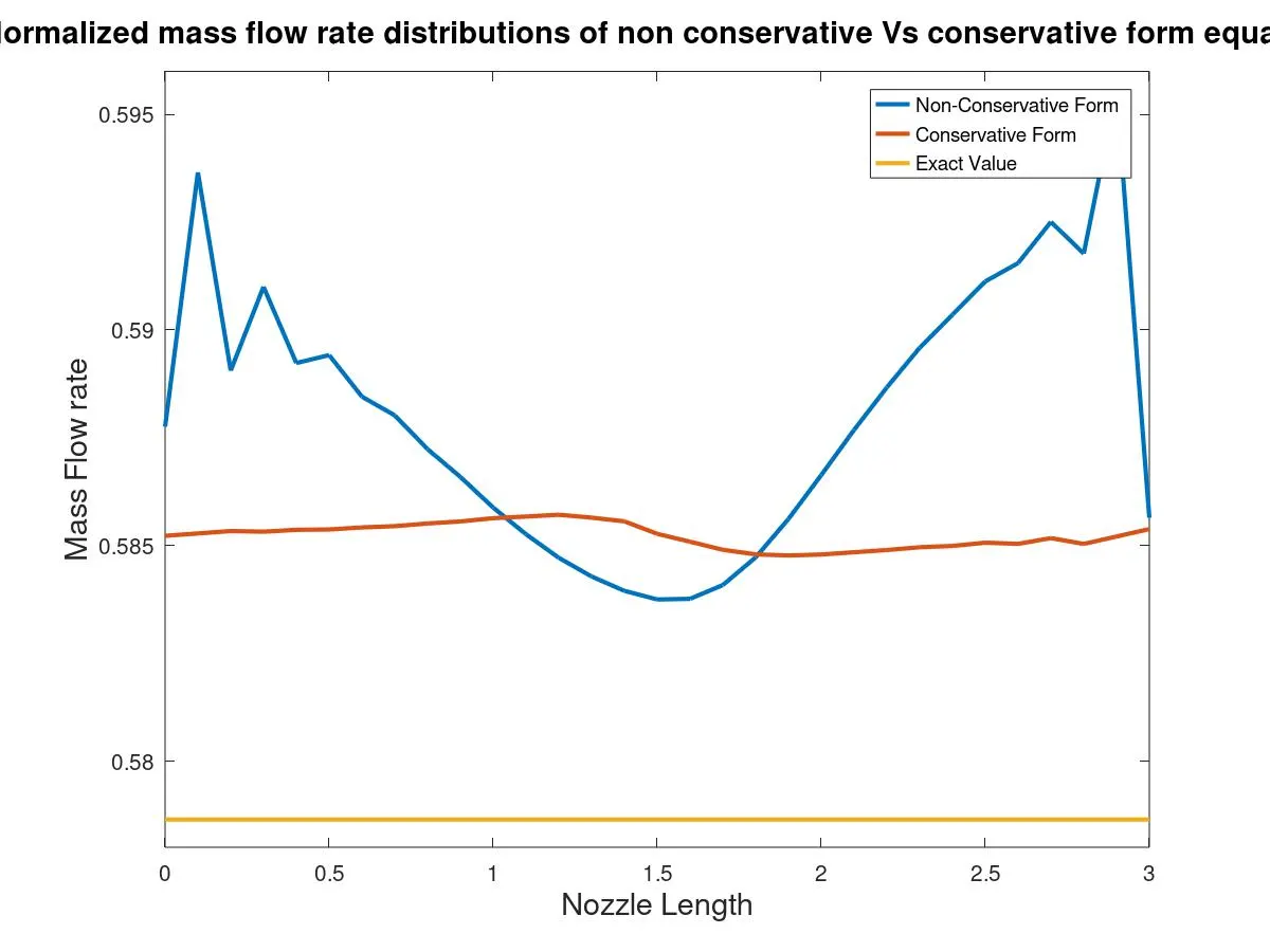
Graph 7

Graph 7 shows the mass flow rate along the nozzle length of Non-conserative form, conservative form and exact value.We can observe that mass flow rate curve of non-conserative form is erratic in nature. The mass flow rate fluctuates at both inlet and outlet and drops down at the throat section whereas in conserative form mass flow rate is almost constant throught the nozzle.

5.2 Non-Conservative form V/s Conservative form with 61 Grid points

1. Steady-state distribution of primitive variables inside the nozzle

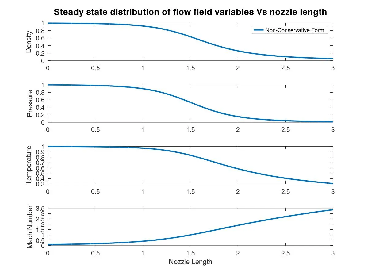
Graph 8

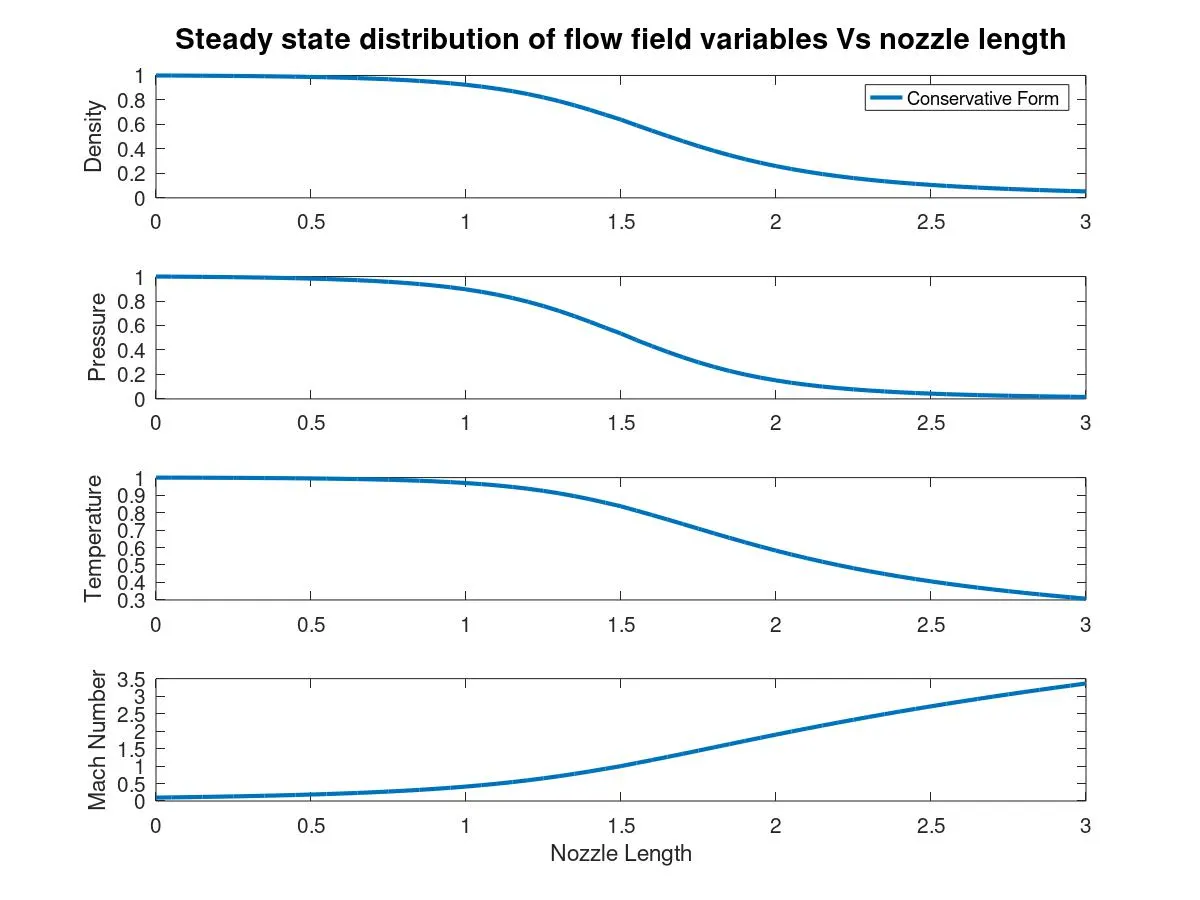
Graph 9

Graph 8 and 9 shows the flow field variables along the nozzle length in non-conservative and conservative form respectively. The behaviour of the curve of each variable is almost same in both forms. There is not much difference when compared to Graph 1 and 2 (31 grids).

2. Time-wise variation of the primitive variables

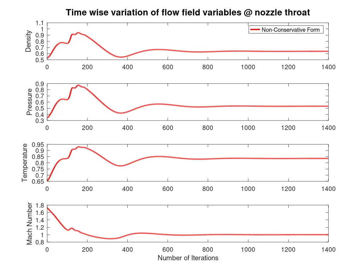
Graph 10

Graph 11

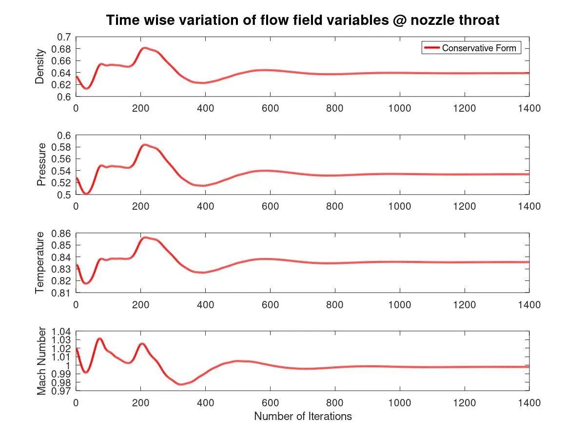
Graph 10 and 11 shows that the time wise variation variation of flow field variables such as Density, Temperature, Pressure and Mach number values at nozzle throat in non-conservative and conservative form respectively. The fluctuation of values is more at the beginning in conservative form than the non- conservative form. The values becomes constant only after around 600 iterations at throat section of CD nozzle (node, i=31) approximately in both forms.

3.Variation of Mass flow rate distribution inside the nozzle at different time steps

Graph 12

Graph 13

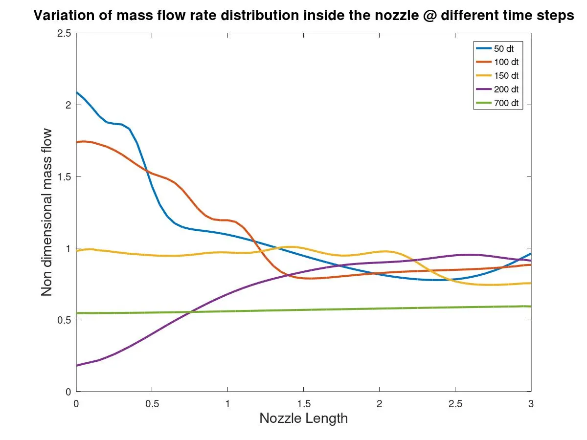
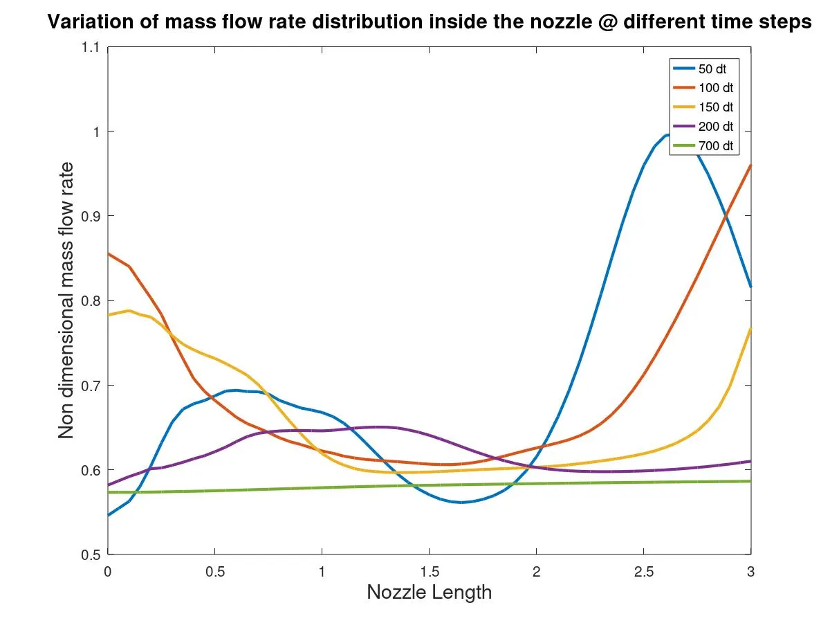
Graph 12 and 13 indicates the mass flow rate along the nozzle length at different time steps in non-conservative and conservative form respectively. We can observe that mass flow rate fluctuates in the beginning and stabilizes after halfway through the nozzle length at all time steps except at 700 time steps in non-conservative form, but the values again shoots up at the outlet in conservative form. The exact mass flow rate values is achived only after 700 time steps in both forms.

4. Comparison of Normalized mass flow rate distributions of both forms

Graph 14

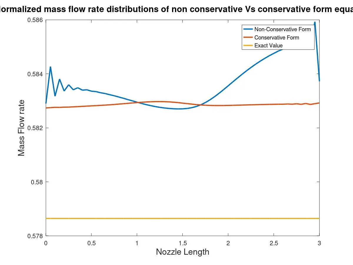
Graph 14 shows the mass flow rate along the nozzle length of Non-conserative form, conservative form and exact value.We can observe that mass flow rate curve of non-conserative form is erratic in nature. The mass flow rate fluctuates at inlet, high at outlet and drops down at the throat section whereas in conserative form mass flow rate is almost constant throught the nozzle.

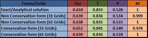
5. Grid independent study – Values from throat section

6. CONCLUSION

1. The above graph shows the comparison between the conservative and non-conservative form while solving the quasi 1D supersonic nozzle flow equation numerically using Mac-Cormack method.
2. CD Nozzle – Subsonic speed in convergent section, Supersonic speed in divergent section and sonic condition at throat is achieved.
3. Stability - The flow field variable plots show that the values are more stable in conservative form than non-conservative form.
4. Mass Flow rate value is closer to exact value in conservative form than non-conservative form.
5. Non-Conservation form can be used if the focus of our solution is primitive variables whereas Conservation form can be used for solution vectors.
6. Grid independence study - Both Non-conservative form & Conservative form are grid independent as the flow field variables remains almost same. But the variations are slightly are higher in conservative form than non-conservative form. But the doubling of number of grids in conservative form leads to faster change of values towards the exact solution than the non-conservative form.
7. Simulation Time - The time taken for the simulation is more in case of non-conservative form than the conservative form.
8. Programming setup - As far as programming and setting up the problem is concerned non-conservative form is much simpler than conservative form.
9. The choice of the form should be made depending on the nature of the problem and purpose of the solution which can come very handy for numerical computation.
10. Overall we can conclude that theoretically there is no difference between conservative and non-conservative form of the equation but a lot of difference lies in numerical discretization process.