Simulation of Laminar Flow over a 2D Backward Facing Step using BlockMesh technique in OpenFOAM

SIMULATION OF LAMINAR FLOW OVER A 2D BACKWARD FACING STEP USING OpenFOAM

1. AIM

Our aim is to simulate a laminar flow over a backward facing step by solving the governing flow equations using OpenFOAM.

2. THEORY/EQUATIONS/FORMULAE USED

OpenFOAM is an open source CFD package. It is a Finite Volume Method (FVM) based tool as it can handle unstructured mesh as well.

It contains basic predefined solvers which can be used to solve our problem, but we need to make sure that correct solver is chosen.

Structure of OpenFOAM simulations

The important directories for a simulation are as follows,

1. System – It consists of various files such as Control Dict, BlockMesh Dict, fv schemes, fv solutions. It defines the mesh and discretization schemes for the simulation.
2. Constant – It consists of various files such as transport properties, boundaries. Polymesh directory is formed after running the blockMesh Dict file.
3. Time directory – It consists folder named 0 before running the simulation. The 0 folder contains files which defines the initial conditions. After running the simulation, the results at every time intervals are also saved here.

OpenFOAM solver – icoFoam is more suitable for backward step facing problem. It solves for velocity and pressure.

3D Geometry - Backward Facing Step

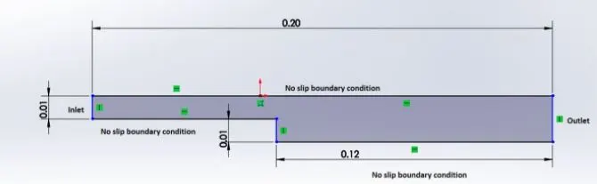
Given inputs

Number of Cells Mesh specification

1. X axis – 200 Grading Factor on the walls – 0.2
2. Y axis – 10

3. OBJECTIVES & PROCEDURE

• The main objective is to simulate a laminar flow over a backward facing step by using OpenFOAM solver and understand the flow behavior for different grading factor.
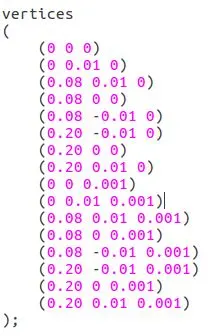
• In the process, firstly the geometry is divided into 3 blocks. Blocks are defined by the vertices of a coordinate system in the blockMesh Dict file.
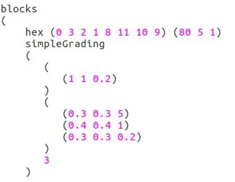
• Mesh grading for all the 3 blocks is defined by multi-grading. Three different cases are defined with grading factor 0.2, 0.5 and 0.8.
• After defining the blocks and grading factor the Polymesh folder is generated and transport property i.e., kinematic viscosity is defined in the constant directory.
• Then the initial and boundary condition are defined as per the problem. The primitive variables such as Velocity and Pressure are calculated using the solver.
• Velocity contours and plot are generated and analyzed.

4. NUMERICAL ANALYSIS (Software used – OpenFOAM 4.1)

• Geometric Modeling

Blocks

The 3D geometry is divided into 3 blocks but it is treated as 2D by not defining any grids on z-axis.

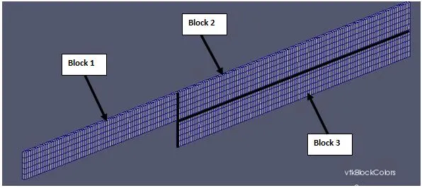
The above figure shows all three 3 blocks and a simple mesh.

Vertices forming all three blocks

MESHING

Mesh - Example for defining block with mesh grading 0.2

Block 1

Block 2

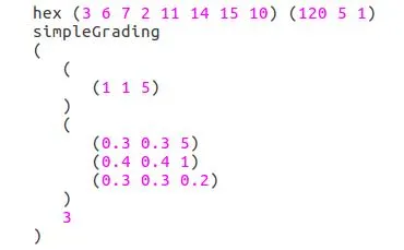
Block 3

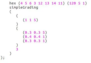
Grading Factor = 0.2

Grading Factor = 0.5

Grading Factor = 0.8

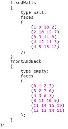
Boundaries

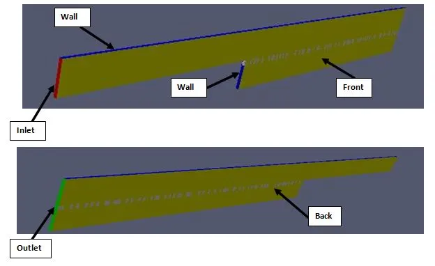
Boundary Condition

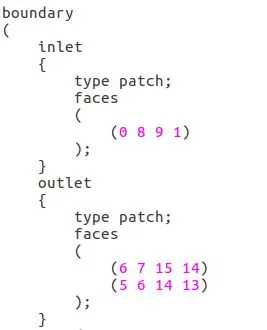
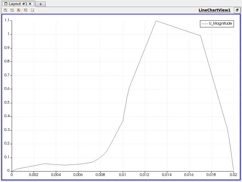
5. RESULTS - Velocity Plot at 0.085 m

1. 0.2 Grading

0.2 velocity plot

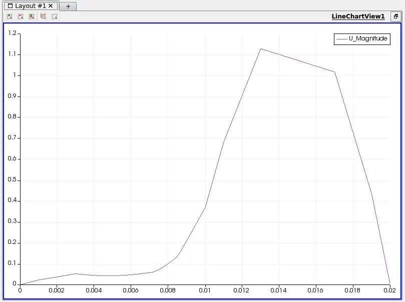
2. 0.5 Grading

0.5 velocity plot

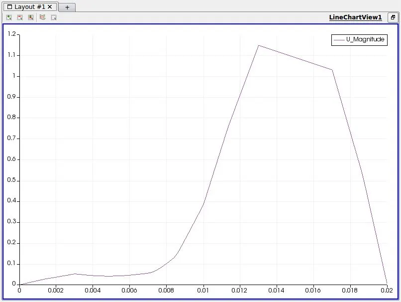
3. 0.8 Grading

0.8 velocity plot

6. CONCLUSION

1. The backward facing step problem is solved for velocity with different mesh grading using icoFoam solver in OpenFOAM.
2. Graph 1,2 & 3 shows the velocity along the y-axis of backward facing step at x=0.085 m of mesh grading 0.2, 0.5 and 0.8 respectively.
3. The distance x is exactly at the step region of the backward facing step where the fluid start comes out of a narrow area.
4. Setup - As far as setting up the problem is concerned, firstly the choice of the solver should be made depending on the nature of the problem and purpose of the solution, then defining the blocks via vertices and mesh grading in blockMesh Dict file is very important before running the solver.
5. Mesh Grading - Different mesh grading near the walls are used to study the behavior i.e., boundary layer. Boundary layer can be seen more clearly with 0.2 grading compared to 0.5 and 0.8 grading.
6. The velocity is less than 0.1 in the first half of the step i.e., between 0 to 0.008m on y-axis. The velocity starts to increase at y=0.01 and achieves the peak velocity of 1.1 to 1.2 at around y=0.013 and then after y=0.017 the velocity drops. The behaviour of the velocity curve of each graph is almost same for this problem.