Week-4 Challenge WOT Condition Part-2

Answer:

1)

Mapped model:

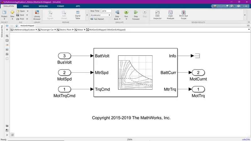
Mapped models of the components are basically representations of the components in the form of lookup tables.

These models take the inputs and the lookup table gives the respective outputs.

The picture below is an example of a mapped model of the motor/generator of an EV.

Dynamic model:

Dynamic models are the actual systematic representations of the components.

They are modeled by the actual knowledge of the components.

The picture below is an example of a dynamic model of the motor/generator of an EV.

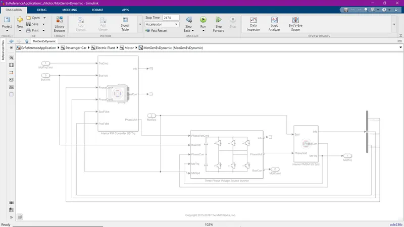
You can see the output of the model is obtained by the actual system of the motor/generator.

To change the model type, double-click the electric plant block.

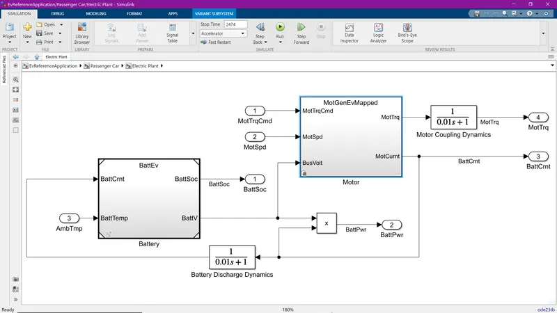
Right-click on the motor block.

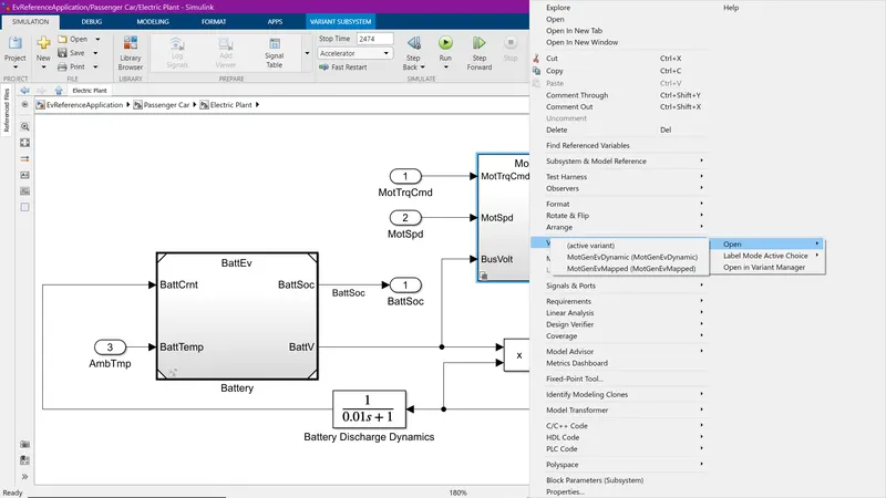
Choose Variant -> Open .

Now you can choose the model type of the component as your wish.

2)

To find how the model calculates miles per gallon of the vehicle, we need to find where these operations are done.

Double-click on the visualization block.

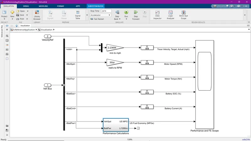
There you can see the performance calculations block where it calculates the fuel economy of the vehicle.

Double-click on the block and you can see how the miles per gallon is calculated.

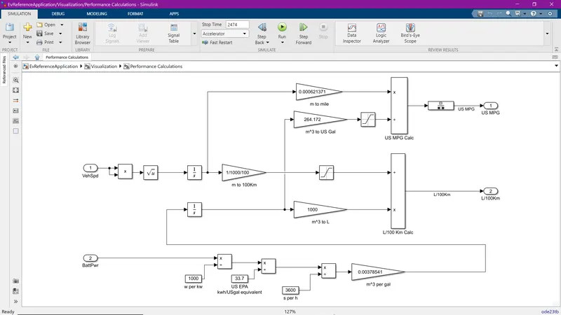
There are two factors considered to model the fuel flow of the vehicle.

They are 1. Vehicle speed 2. Battery power

The vehicle speed is converted to distance by integration and the battery power is converted to gallons by some calculations. Now, this distance is divided by the gallons which give the miles per gallon of the vehicle.

3)

To open up the HEV ReferenceApplication, the command 'autoblkHevStart' is typed in the command window.

The model is popped up.

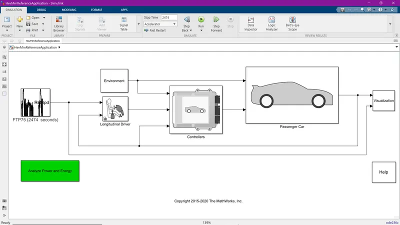
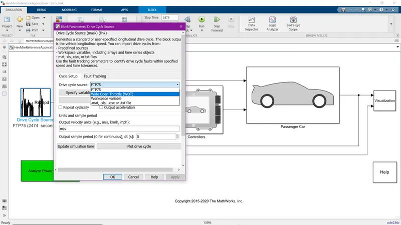
To change the drive cycle, double-click on the Drive cycle block and a dialog box is opened.

In the dialog box, change the drive cycle source to Wide Open Throttle(WOT), and update the simulation time, while keeping the rest of the parameters default, click Apply and then OK.

To change the grade and wind velocity, double-click on the Environment block.

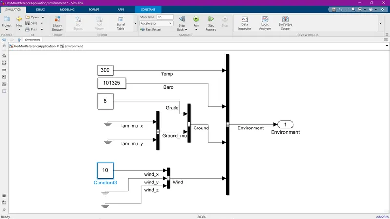
The grade is changed to '8' and the wind speed is changed to 10 m/s.

Now, with the updated model, the simulation is started with the updated simulation time(i.e,) 30 seconds.

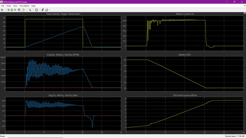
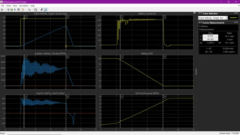
It is seen that the vehicle achieved a trace velocity of 67.1 mph and an actual velocity of 48. 7 mph(due to grade).

Since we add grade and wind speed to the vehicle, the motor should deliver high torque (Max. Torque = 300 Nm achieved) in order for the movement.

It is seen that the motor delivers high torque during the run and thus the high speed (Max. speed = 9000 rpm achieved).

When deceleration, the motor torque becomes negative.

Since the motor is run by a battery, the battery delivers a large amount of current (Max. current = 528 A achieved).

The battery draws the current during the run, so the SOC of the battery gradually drops from 80 to 70.

Max. Fuel Economy achieved is 7.4.

4)

To open up the EV ReferenceApplication, the command 'autoblkEvStart' is typed in the command window.

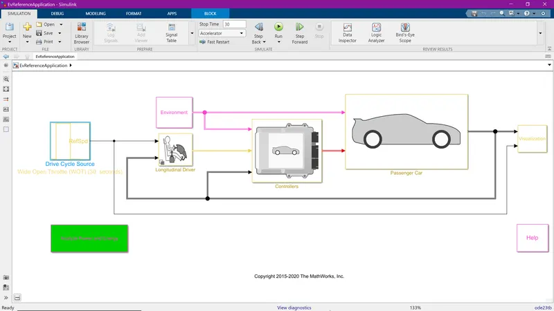
The model is set with the same parameters as in the above simulation.

The model is run and the results are shown below.

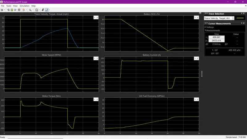
HEV results for quick reference:

Comparison:

1) In the case of EV, The battery draws a high current but the SOC of the battery decrease only a little.

2) Fuel economy of the EV(14) is higher than that of the HEV.

3) Motor speed is lesser in an EV(5000 rpm).

4) EV achieved a top speed of 45.8 mph which is lower than that of an HEV.