Week-4 Challenge WOT Condition Part-2
- What is the difference between mapped and dynamic model of engine, motor and generator? How can you change model type?
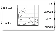
Ans: Mapped model
1) In mapped model data points are pre-assigned in lookup table which would be configured with the operational parts and the analysis would be formed
. 2) Model uses a set of steady-state lookup tables to characterize engine performance
3) The accuracy is low for this system.
4) Run time simulaion less time,because it does not run with real time simulation.
Dynamic model
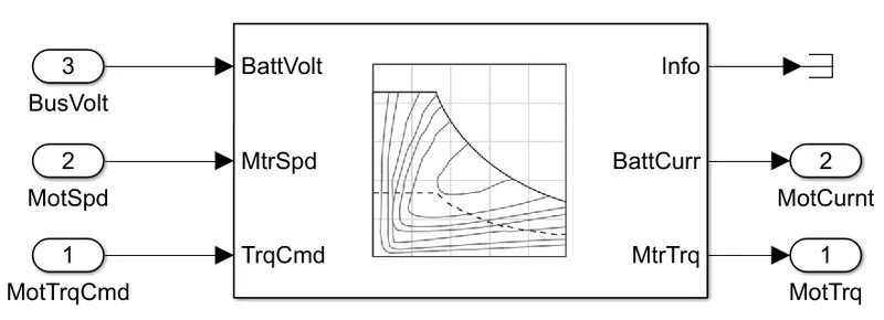
- Dynamic engines decompose engine behavior into individual component models that account for engine dynamics, most notably intake airflow and turbocharger dynamics. You can switch between engine model types based on your application.
1)Dynamic model runs by real time simulator.
2) dynamic model uses the combination of ouput from various subsystem to generate output.
3) The accuracy of dynamic model is very high.
4) Run time simulation take more time.
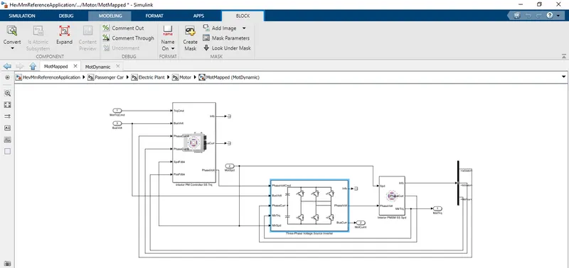
Step to change moel:
1) select vehicle type power train blockset model.
2)Go to passenger block simulink model of electric motor and generator.
3) Right click on block and go to variance label mode active choice motorgen ev mapped or dynamic.
Que:2 How does the model calculated mile per gallon ? which factor are consider for model to fuel flow?
- Fuel flow Battery power are the things that to be considered to model fuel flow. Miles per gallon gasoline equivalent is a measure of the average distance traveled per unit of energy consumed. The miles per gallon is calculated by considering the battery output, Fuel output and speed of vehicle in kilometers driven.
Miles per gallon(MPG)
MPG is a fuel economy ratingdetermined by how far a car can travel on a gallon of gasoline or diesel . although the metric versiuon would be in kmper liters MPGT is adopted in many metric system countries, like canada UK.
While it is cheaper and better for the enviornment to achieve a higher MPG rating, there is a curve, that the EPA called the ''MPG illusion that so the cost benifitsof increasing MPG decreasewith higher RATING.
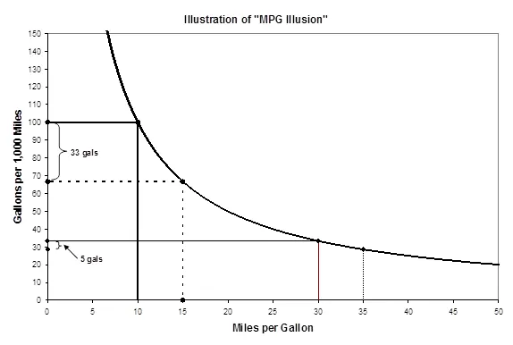
the graph above show MPG illusion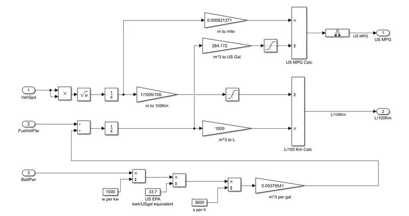
The model calculated the MPG& L/100km by considering the vehicle speed,fuel volume flow& battery power as input.
The input for the US MPG calculation are vehicle speedin miles & fuel flow volume in US gallon.
Factor that effect the fuel Economy:
1) Excessive short trip
2) Frequent cold weather travel
3)Havy braking ands acceleration
4) High speed weight and Towing weight
5)Speeding.
Que:3 Run the HEV ReferenceApplication with WOT drive cycle. Change the grade and wind velocity in the environment block. Comment on the results.h
Ans:
" HEV Refrence Application"
The hybride electric vehicle refrence application represent t6o full multimode hybride electric vehicle (HEV) model with an internal combution engine ,transmission ,battery ,motor ,generator ,and associated powertrain control algorithms, uses the refrence application for powertrain matching analysis and component selection ,control and dignostics algoritham design and hardware - in -the - loop (HIL) testing .
by default, the multimode reference application is configured with :
- Mapped motor and generator
- 1.5-L spark-ignite (SI) dynamic engine
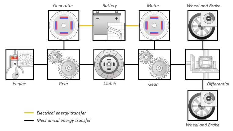
This diagram show the powertrain configuration .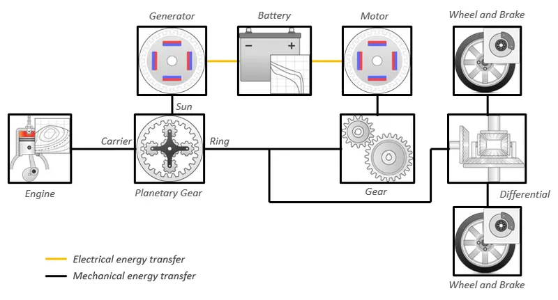
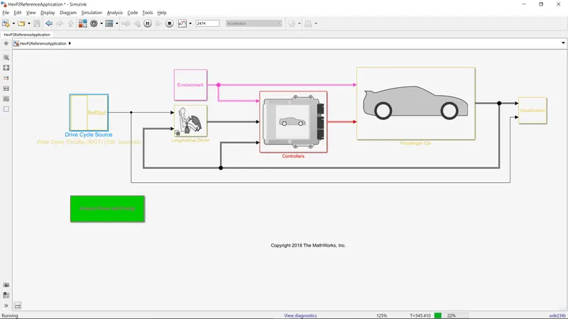
Description:
1) Open HEV reference application model in MATLAB.
2) it consist of various subsystem which are simulate to EV refrence application but the complecty is more in '"HEV Reference Application'model
change the grade and velocity :
.
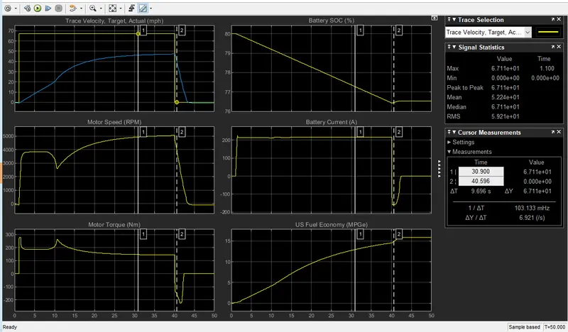
After that . i run the model for 50 sec we can see the picture below :
Result:
Performane and EF Scope:
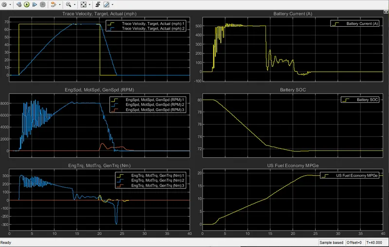
As we can see in the above picture, in plot we applied WOT with applied with velocity within no time , the trace velocity remained 67.1m/h deacceleration. but as we can see the actual velocvity of did not reach the trace velocity because of gradibility and wind .
velocity has been incresed , the value of currunt and engine power is also limited , as we can see in second plot the currunt is going to negative after starting deaccelaration . this negative currunt means the battery is charging and the regenrative brake is applied , we can also see in plot the speed of the motor and generator is same and it overlap .
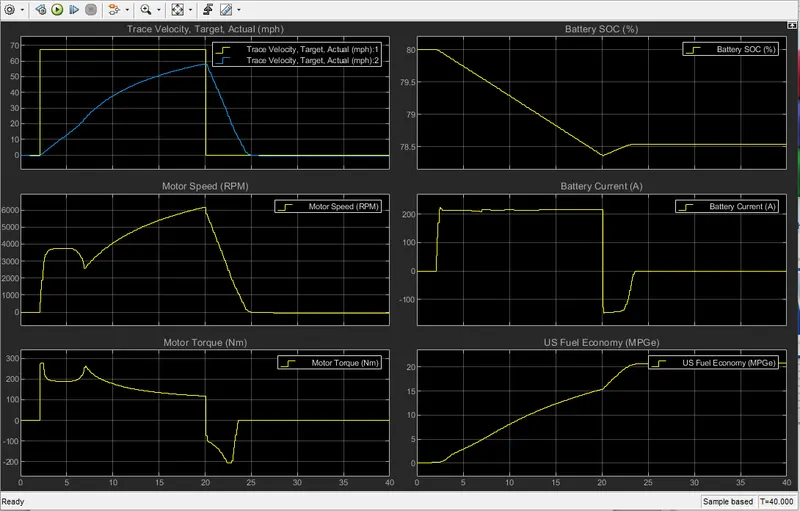
Que4: Keeping all other parameters same, compare the simulated results of hybrid and pure electric powertrain.
The hybrid electric vehicle reference application represents a full multimode hybrid electric vehicle (HEV) model with an internal combustion engine, transmission, battery, motor, generator, and associated powertrain control algorithms. Use the reference application for powertrain matching analysis and component selection, control and diagnostic algorithm design, and hardware-in-the-loop (HIL) testing. To create and open a working copy of the hybrid electric vehicle reference application project, enter
By default, the HEV multimode reference application is configured with:
-
Mapped motor and generator
-
1.5–L spark-ignition (SI) dynamic engine
This diagram shows the powertrain configuration.
This table describes the blocks and subsystems in the reference application, indicating which subsystems contain variants. To implement the model variants, the reference application uses variant subsystems.
| Reference Application Element | Description | Variants |
|---|---|---|
|
Analyze Power and Energy |
Double-click Analyze Power and Energy to open a live script. Run the script to evaluate and report power and energy consumption at the component- and system-level. For more information about the live script, see |
NA |
|
Drive Cycle Source block — FTP75 (2474 seconds) |
Generates a standard or user-specified drive cycle velocity versus time profile. Block output is the selected or specified vehicle longitudinal speed. |
✓ |
|
|
Creates environment variables, including road grade, wind velocity, and atmospheric temperature and pressure. |
|
|
|
Uses the Longitudinal Driver or Open Loop variant to generate normalized acceleration and braking commands.
|
✓ |
|
|
Implements a powertrain control module (PCM) containing a hybrid control module (HCM) and an engine control module (ECM). |
✓ |
|
|
Implements a hybrid passenger car that contains engine, electric plant, and drivetrain subsystems. |
✓ |
|
|
Displays vehicle-level performance, battery state of charge (SOC), fuel economy, and emission results that are useful for powertrain matching and component selection analysis. |
Evaluate and Report Power and Energy
Double-click Analyze Power and Energy to open a live script. Run the script to evaluate and report power and energy consumption at the component- and system-level. For more information about the live script,
The script provides:
-
An overall energy summary that you can export to an Excel® spreadsheet.
-
Engine plant, electric plant, and drivetrain plant efficiencies, including an engine histogram of time spent at the different engine plant efficiencies.
-
Data logging so that you can use the Simulation Data Inspector to analyze the powertrain efficiency and energy transfer signals.
Drive Cycle Source
The Drive Cycle Source block generates a target vehicle velocity for a selected or specified drive cycle. The reference application has these options.
| Timing | Variant | Description |
|---|---|---|
|
Output sample time |
|
Continuous operator commands |
|
|
Discrete operator commands |
Longitudinal Driver
The Longitudinal Driver subsystem generates normalized acceleration and braking commands. The reference application has these variants.
|
Block Variants |
Description | ||
|---|---|---|---|
|
Longitudinal Driver (default) |
Control |
|
PI control with tracking windup and feed-forward gains that are a function of vehicle velocity. |
|
|
Optimal single-point preview (look ahead) control. |
||
|
|
Proportional-integral (PI) control with tracking windup and feed-forward gains. |
||
|
Low-pass filter (LPF) |
|
Use an LPF on target velocity error for smoother driving. |
|
|
|
Do not use a filter on velocity error. |
||
|
Shift |
|
Stateflow® chart models reverse, neutral, and drive gear shift scheduling. |
|
|
|
Input gear, vehicle state, and velocity feedback generates acceleration and braking commands to track forward and reverse vehicle motion. |
||
|
|
No transmission. |
||
|
|
Stateflow chart models reverse, neutral, park, and N-speed gear shift scheduling. |
||
|
Open Loop |
Open-loop control subsystem. In the subsystem, you can configure the acceleration, deceleration, gear, and clutch commands with constant or signal-based inputs. |
||
To idle the engine at the beginning of a drive cycle and simulate catalyst light-off before moving the vehicle with a pedal command, use the Longitudinal Driver variant. The Longitudinal Driver subsystem includes an ignition switch signal profile, IgSw. The engine controller uses the ignition switch signal to start both the engine and a catalyst light-off timer.
The catalyst light-off timer overrides the engine stop-start (ESS) stop function control while the catalyst light-off timer is counting up. During the simulation, after the IgSw down-edge time reaches the catalyst light-off time CatLightOffTime, normal ESS operation resumes. If there is no torque command before the simulation reaches the EngStopTime, the ESS shuts down the engine.
To control ESS and catalyst light-off:
-
In the Longitudinal Driver Model subsystem, set the ignition switch profile
IgSwto 'on'. -
In the engine controller model workspace, set these calibration parameters:
-
EngStopStartEnable— Enables ESS. To disable ESS, set the value to false. -
CatLightOffTime— Engine idle time from engine start to catalyst light-off. -
EngStopTime— ESS engine run time after driver model torque request cut-off.
-
Controllers
The Controller subsystem has a PCM with an HCM and an ECM.
ECM
The reference application has these variants for the ECM.
| Controller | Variant | Description |
|---|---|---|
| ECM | SiEngineController (default) |
SI engine controller |
CiEngineController |
CI engine controller |
HCM
The HCM implements a dynamic embedded controller that directly determines the engine operating point that minimizes brake-specific fuel consumption (BSFC) while meeting or exceeding power required by the battery charging and vehicle propulsion subsystems.
To calculate the optimal engine operating point in speed and torque, the controller starts with a candidate set of discrete engine power levels. For each power level candidate, the block has a parameterized vector of torque and speed operating points that minimize BSFC.
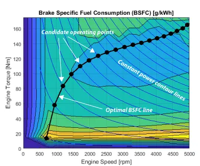
The optimizer then removes power level candidates that are unacceptable for either of these reasons:
-
Too much power sent through the generator to the battery.
-
Too little power to meet charging and propulsion subsystem requirements.
Of the remaining power level candidates, the controller selects the one with the lowest BSFC. The controller then sends the associated torque / speed operating point command to the engine.
Passenger Car
To implement a passenger car, the Passenger Car subsystem contains drivetrain, electric plant, and engine subsystems. To create your own engine variants for the reference application, use the CI and SI engine project templates. The reference application has these subsystem variants.
Drivetrain
| Drivetrain Subsystem | Variant | Description | |
|---|---|---|---|
|
Differential and Compliance |
All Wheel Drive |
Configure drivetrain for all wheel, front wheel, or rear wheel drive. For the all wheel drive variant, you can configure the type of coupling torque. |
|
Front Wheel Drive (default) |
|||
Rear Wheel Drive |
|||
|
Vehicle |
Vehicle Body 3 DOF Longitudinal |
Configured for 3 degrees of freedom |
|
|
Wheels and Brakes |
|
For the wheels, you can configure the type of:
For performance and clarity, to determine the longitudinal force of each wheel, the variants implement the Longitudinal Wheel block. To determine the total longitudinal force of all wheels acting on the axle, the variants use a scale factor to multiply the force of one wheel by the number of wheels on the axle. By using this approach to calculate the total force, the variants assume equal tire slip and loading at the front and rear axles, which is common for longitudinal powertrain studies. If this is not the case, for example when friction or loads differ on the left and right sides of the axles, use unique Longitudinal Wheel blocks to calculate independent forces. However, using unique blocks to model each wheel increases model complexity and computational cost. |
|
|
|
|||
Electric Plant
| Electric Plant Subsystem | Variant | Description |
|---|---|---|
| Battery | BattHevMm (default) |
Configured with electric battery |
| Generator | GenMapped (default) |
Mapped generator |
GenDynamic |
Interior permanent magnet synchronous motor (PMSM) with controller |
|
| Motor | MotMapped (default) |
Mapped motor with implicit controller |
MotDynamic |
Interior permanent magnet synchronous motor (PMSM) with controller |
Engine
| Engine Subsystem | Variant | Description | |
|---|---|---|---|
| Engine |
|
Dynamic SI engine with turbocharger |
|
|
|
Dynamic naturally aspirated SI Core Engine |
||
|
|
Dynamic SI V Twin-Turbo Single-Intake Engine |
||
|
|
Dynamic SI V Engine |
||
|
|
Dynamic SI V Twin-Turbo Twin-Intake Engine |
||
|
|
Mapped SI engine with implicit turbocharger |
||
|
|
Deep learning SI engine |
||
|
|
Dynamic core SI engine with turbocharger |
||
|
|
Mapped CI engine with implicit turbocharger |
||