Week-4 Challenge WOT Condition Part-2

1.What is the difference between mapped and dynamic model of engine, motor and generator.

Powertrain blockset:

Powertrain Blockset provides fully assembled reference application models of automotive powertrains, including gasoline, diesel, hybrid, and electric systems. It includes a component library for simulating engine subsystems, transmission assemblies, traction motors, battery packs, and controller models. Powertrain Blockset also includes a dynamometer model for virtual testing. MDF file support provides a standards-based interface to calibration tools for data import.

Powertrain Blockset provides a standard model architecture that can be reused throughout the development process. You can use it for design tradeoff analysis and component sizing, control parameter optimization, and hardware-in-the-loop testing. You can customize models by parameterizing components in a reference application with our data or by replacing a subsystem with our model.

Reference applications serve as a starting point for our system model. To tailor a reference application to your powertrain project, parameterize the components in the reference application using data from a domain-specific tool, a test bench, or a vehicle. Depending on your application and powertrain configuration, you might need to select the type of component models and further customize the system model.

Powertrain Blockset provides a set of fully assembled reference applications, including gasoline (spark-ignition, SI), diesel (compression-ignition, CI), hybrid, and electric vehicle systems, as a starting point for your powertrain system model. To model a powertrain system for your project, you can select a reference application based on the powertrain type. Each reference application includes plant models, controllers, a longitudinal driver, and drive cycle data.

The component library in Powertrain Blockset provides blocks of physical systems and controllers for:

• Propulsion
• Transmission
• Drivetrain
• Energy storage
• Longitudinal vehicle dynamics
• Drive cycle data and longitudinal driver

All the models in Powertrain Blockset, including the reference applications and components in the library, are fully open for customization. You can use Simulink Projects to manage model variants including variant selection, version management, and comparison.

Powertrain Blockset provides two types of combustion engine models: mapped and dynamic. Mapped engines represent macro engine behaviour as a set of lookup tables (brake torque, fuel flow, air mass flow, exhaust temperature, efficiency, and emissions) as functions of commanded load and measured engine speed. Dynamic engines decompose engine behaviour into individual component models that account for engine dynamics, most notably intake airflow and turbocharger dynamics.

You can switch between engine model types based on your application. Dynamic engine models are suitable for designing control, estimator, and diagnostic algorithms that depend on dynamic subsystem states, for example, in closed-loop AFR control algorithm development. Mapped engine models are suitable for analysis and design activities that do not require engine subsystem dynamic characteristics, for example, in engine and transmission powertrain matching analysis for fuel economy, emissions, and performance tradeoffs.

Both the SI and CI engine models run in real time for Hardware-in-loop(HIL) testing.

Mapped model:

Mapped model represent the macro behaviour of the subsystem as a set of lookup tables. these models are useful for understanding the behaviour of the subsystem using empirical data.it reduces the complexity of simulations as it uses data to simulate the model .but in mapped model data has to be collected and fed into the model.

Dynamic model:

Dynamic model decompose the subsystem behaviour into individual component models. it dynamically adjusts to the operation giving us a detailed analysis of the components of the model .but dynamic models are difficault to build for customized operations.

MAPPED MODEL ENGINE:

Mapped engine models are suitable for analysis and design activities that do not require engine subsystem dynamic characteristics, for example, in engine and transmission powertrain matching analysis for fuel economy, emissions, and performance tradeoffs. Both the SI and CI engine models run in real time for hardware-in-the-loop (HIL) testing.

Dynamic model engine:

These are used to decompose the engine behaviour into smaller individual component models that account for engine dynamics, intake airflow, and turbocharger dynamics.

Dynamic engines are used when we have component-level data.

This block calculates the fuel flow, air mass flow, air-fuel ratio, and exhaust mass flow rate.

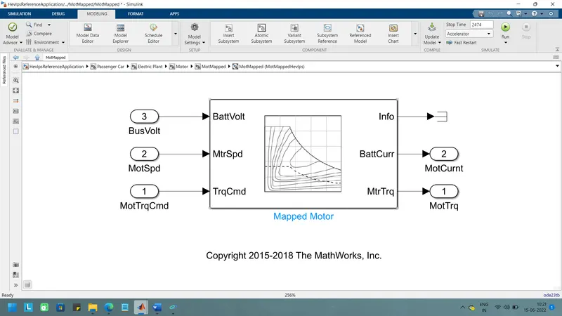
MAPPED MODEL MOTOR:

The Mapped Motor block implements a mapped motor and drive electronics operating in torque-control mode. The output torque tracks the torque reference demand and includes a motor-response and drive-response time constant.

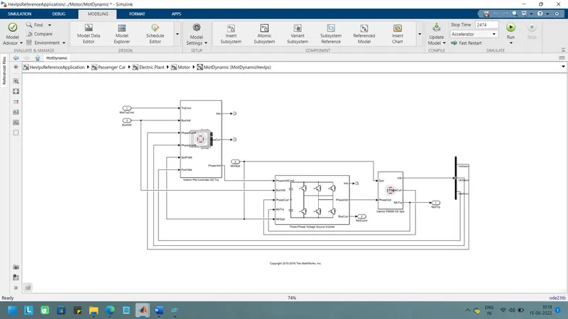
Dynamic model motor:

This model is used when all the parameters are known. So here the actual specifications of the motor are considered and the result is simulated. This motor uses a torque-based field controller for an internal permanent magnet synchronous machine with an optional output loop speed controller. These are more accurate when compared to the mapped motors.

MAPPED MODEL GENNERATOR:

In this model, we have to give the specifications of battery torque, battery current, and others in the lookup table before simulating the result. Results are given based on the data interpreted.

Dynamic model generator:

It performs a real-time simulation of components that takes place in the real system. In the model, simulation gives a detailed analysis.

How can you change model type?

We can switch the mapped model to dynamic model as per our requirement.

• open the powertrain module blockset for required vehicle
• open the passenger car/electric plant/motor
• click the right button to motor subsystem in that subsystem & odel reference and select convert to variant

Before changing mapped to dynamic as shown below.

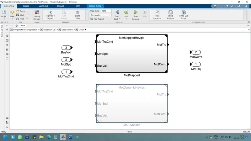
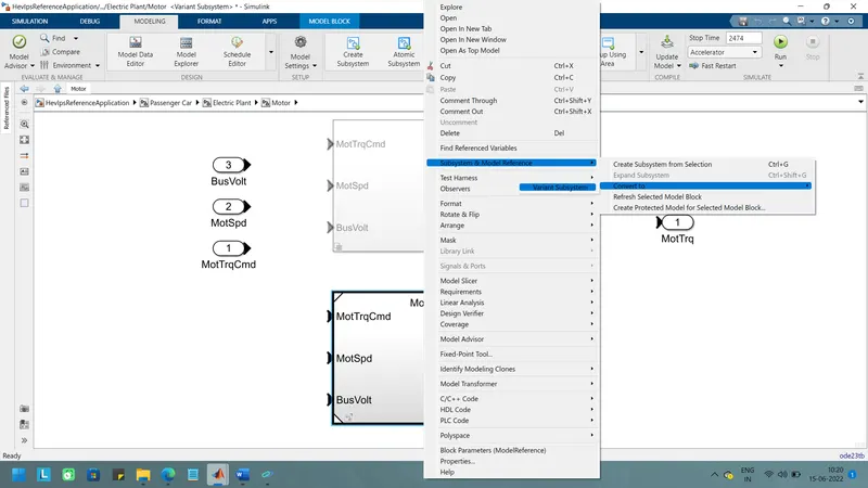
then open model explorer change lable as mapped to dynamic.

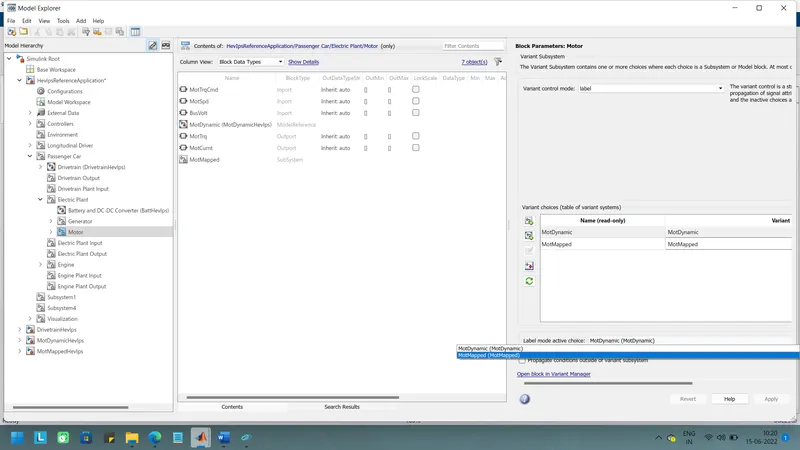
After changing the mapped to dynamic as shown below.

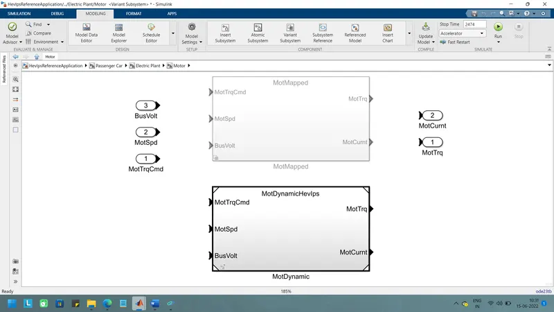
2.

Miles per gallon:

it is a fuel economy rating determined by how far a car can travel using one gallone of gasoline or diesel for a conventional IC engine type.in the caase of an electric vehicle, this is a measure of how much electrical energy is consumed by the battery pack to travel a fixed distance.

The model takes an input of vehicle speed, fuel flow, battery power to calculate the fuel consumption and bateery consumption and to calculate the miles per gallon.

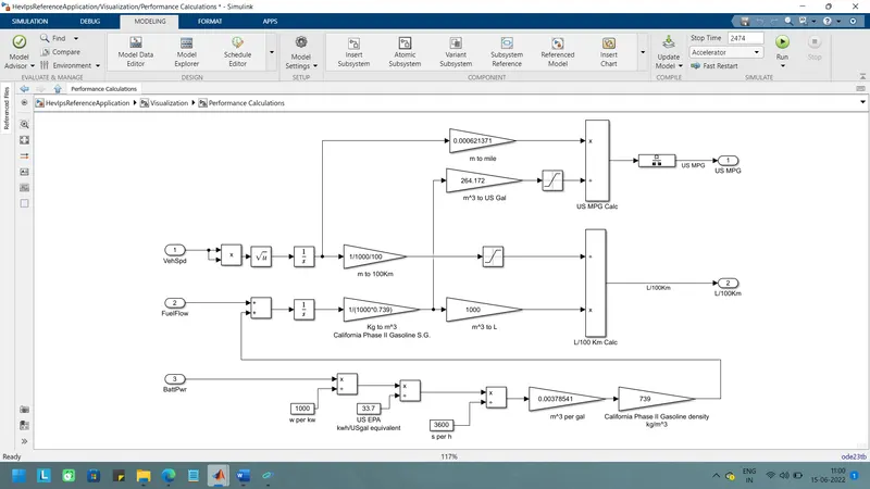
Calculating the miles per gallon:

• The inputs from the vehicle (i.e,) the distance found in meters so we convert it into miles by multiplying with 0.0006213
• Then the inputs from fuel flow( battery power+fuel energy) taken in m^3 and are converted into us gallon by multiplying with 264.172.
• Battery power is in watts so we can convert it into kw by deviding with 1000 and it is converted into us gallon of automotive gasoline by deviding with 33.7 so it gets kwh to get the energy in us gallon per seconds we devide with 3600 and we convert the hours to seconds.
• Then multiplying with 0.00378541 converting the us gallon per sec to volume of the fuel flow in m^3/s.
• Then multiplying with 739 (california phase|| gasoline densitykg/s).
• The result is got in miles per gallon.

Factors considerd in the fuel flow are

• Fuel economy
• Fuel consumption

Majour factors considerd in the fuel economy are

• Vehicle speed
• Engine speed
• Motor torque

Fuel consumption is the amount of fuel consumed in driving a given distance.

3 a)

A hybrid electric vehicle (HEV) is a type of hybrid vehicle that combines a conventional internal comburstion engine (ICE) system with an electric propulsion system (hybrid vehicle drivetrain). The presence of the electric powertrain is intended to achieve either better fuel economy than a conventional vehicle or better performance. There is a variety of HEV types and the degree to which each function as an electric vehicle (EV) also varies.

The hybrid electric vehicle (HEV) input power-split reference application represents a full HEV model with an internal combustion engine, transmission, battery, motor, generator, and associated powertrain control algorithms. Use the HEV input power-split reference application for HIL testing, tradeoff analysis, and control parameter optimization of a power-split hybrid like the Toyota Prius. To create and open a working copy of the HEV input power-split reference application project.

Architecture of HEV is shown below.

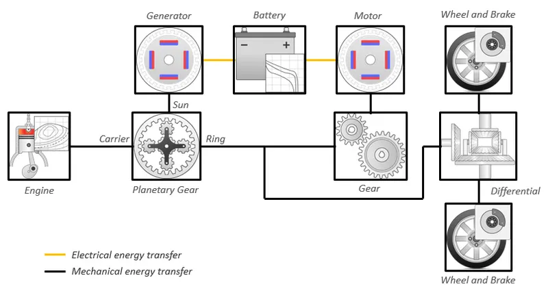
select the file from powertrain blockset in matlab

and enter a below code in matlab

autoblkHevStart

simulation model is shown below.

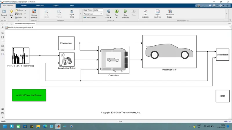
case 1

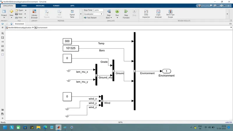
Then changing the FTP drive cycle to WOT drive cycle by clicking the block parameters of drive cycle. keeping grade as 0 and wind velocity as 0 and other parameters as default.

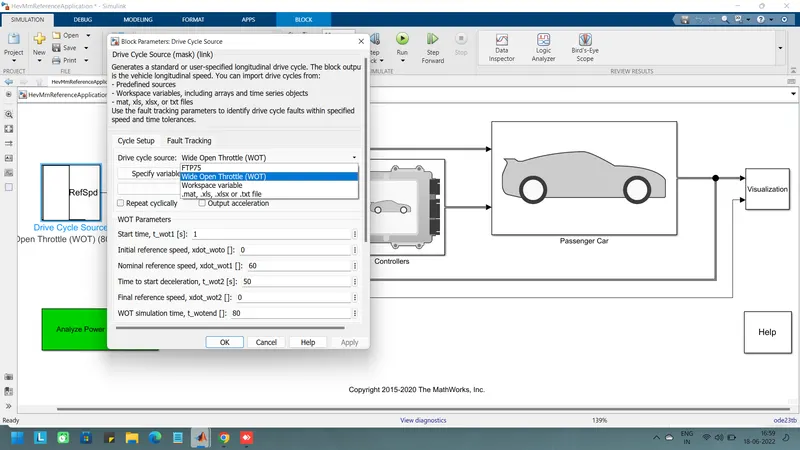
The grade angle=0 degree

The wind velocity =0 m/s

Results

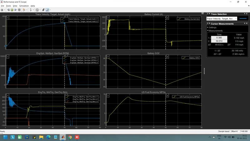
The above results shows results of the simulation and it consists of six plots.

Coursor measurement is helps in reading results in better way.

Plot 1: Trace velocity, Target & Actual(mph)

It shows the velocity of the drive cycle data with the time scale on x-axis.

top speed achived=115mph

The accceleration time to reach the 115 mph = 49.633 sec

the decceleration time from 115 mph to minimum =6.6 sec

Plot 2: Engine speed, Motor speed & Generator speed

It shows the changes in the speed of the engine, motor and generator in rpm through out the drive cycle.

peak engine speed = 5068 rpm

peak motor speed =13892 rpm

Peak generator speed = 5068 rpm

Plot 3: Engine torque, Motor torque & Generator torque

It shows the changes in the torque of the engine, motor and generator in rpm through out the drive cycle.

peak engine torque = 170nm

peak motor torque =307 nm

Peak generator torque = 170 nm

A negative value for the generator indicates the engine torue is used to charge the battery as well during the propulsion time.

Plot 4:Battery current(A)

it shows the battery current values (A) and its changes for various acceleration inputs as per the drive cycle.

The peak current discharge from the battery = 190A

The peak current charging to the battery = -207A

A negative battery current value indicates regenerative braking and charging by the engine.

Plot 5:Battery SOC

It shows the battery state of charge SOC(%) and its changes corresponding to the driving inputs.

The state of charge decreased from 80% to 62% of charge in 48.5 sec ,for the specified driving conditions.

Plot 6: US fuel economy MPGe

It shows the fuel economy as miles per gallons for the corresponding input driving conditions.

3 b) Change the grade and wind velocity in the environment block. Comment on the results.

simulation model

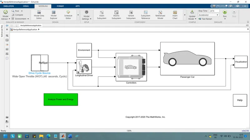
Case 2

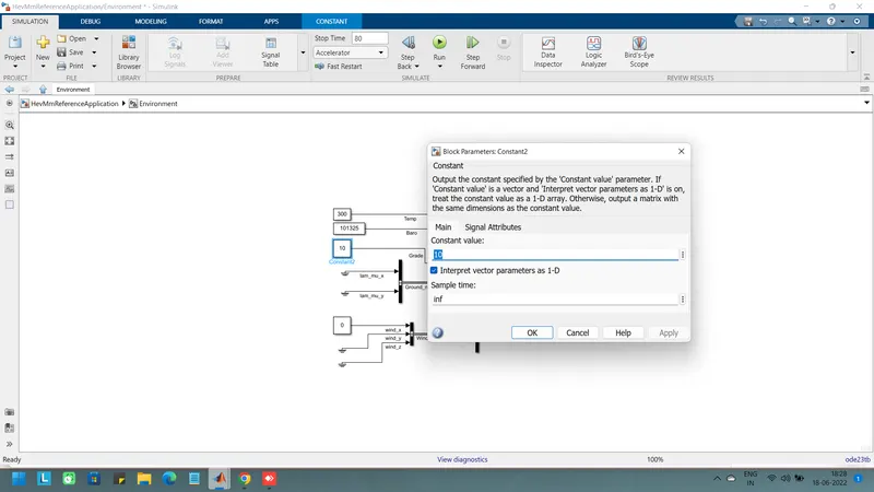
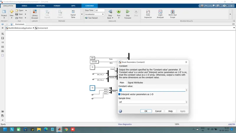
Then changing the FTP drive cycle to WOT drive cycle by clicking the block parameters of drive cycle. Changing the grade and wind velocity in the environment block remaining all parameters as default.

The grade angle=10 degree

The wind velocity =15 m/s

Results

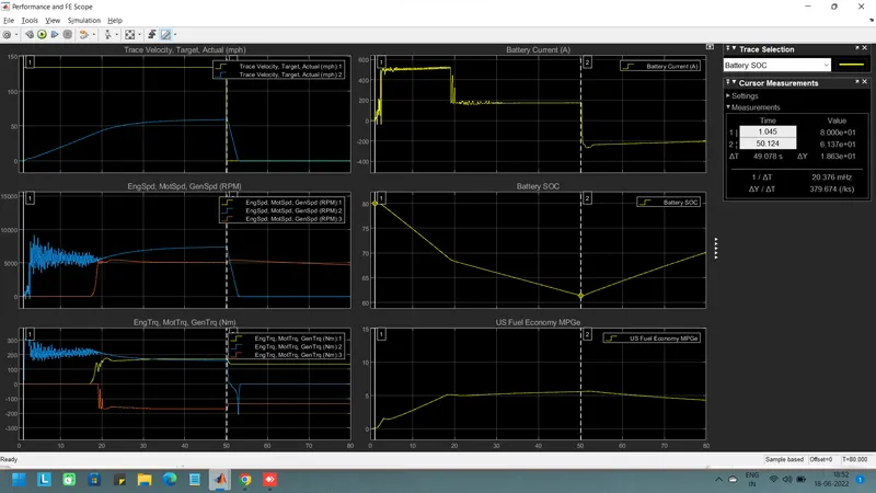
The above results shows results of the simulation and it consists of six plots.

Coursor measurement is helps in reading results in better way.

Plot 1: Trace velocity, Target & Actual(mph)

It shows the velocity of the drive cycle data with the time scale on x-axis.

top speed achived=59.5mph

The accceleration time to reach the 59.5 mph = 49.0sec

the decceleration time from 59.5 mph to minimum =3.9sec

Plot 2: Engine speed, Motor speed & Generator speed

It shows the changes in the speed of the engine, motor and generator in rpm through out the drive cycle.

peak engine speed = 5068rpm

peak motor speed =7368 rpm

Peak generator speed = 5068 rpm

Plot 3: Engine torque, Motor torque & Generator torque

It shows the changes in the torque of the engine, motor and generator in rpm through out the drive cycle.

peak engine torque = 170nm

peak motor torque =305 nm

Peak generator torque = 169 nm

A negative value for the generator indicates the engine torue is used to charge the battery as well during the propulsion time.

Plot 4: Battery current(A)

It shows the battery current values (A) and its changes for various acceleration inputs as per the drive cycle.

The peak current discharge from the battery = 195A

The peak current charging to the battery = -210A

A negative battery current value indicates regenerative braking and charging by the engine.

Plot 5:Battery SOC

It shows the battery state of charge SOC(%) and its changes corresponding to the driving inputs.

The state of charge decreased from 80% to 62% of charge in 49.63 sec ,for the specified driving conditions.

Plot 6: US fuel economy MPGe

It shows the fuel economy as miles per gallons for the corresponding input driving conditions.

Conclusion:

According to the simulation results for with and with out grade angle & wind velocity.

• case 2 due to wind velocity and gradeability, the vehicle is not able to match the targeted speed.
• case 2 max RPM achived by the motor is less beacuse of resistance offered by the grade and wind velocity.
• Battery current is almost same. and battery has same capacity in both the cases.
• State of charge is also discharges as compared to case 1
• MPGe achived less in case 2 than the case 1.
• so overall we can adding wind velocity & gradeability causes the vehicle to achive less acceleration & top speed at same battery capacity & MPGeachives is also less.
• Efficiency of no load vehicle is high compared loads acting on the vehicle.

4. Pure Electric Vehicle

The electric vehicle reference application represents a full electric vehicle model with a motor-generator, battery, direct-drive transmission, and associated powertrain control algorithms. Use the electric vehicle reference application for powertrain matching analysis and component selection, control and diagnostic algorithm design, and hardware-in-the-loop (HIL) testing.

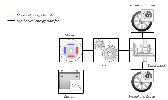
select the file from powertrain blockset in matlab

and enter a below code in matlab

autoblkEvStart

simulation model is shown below.

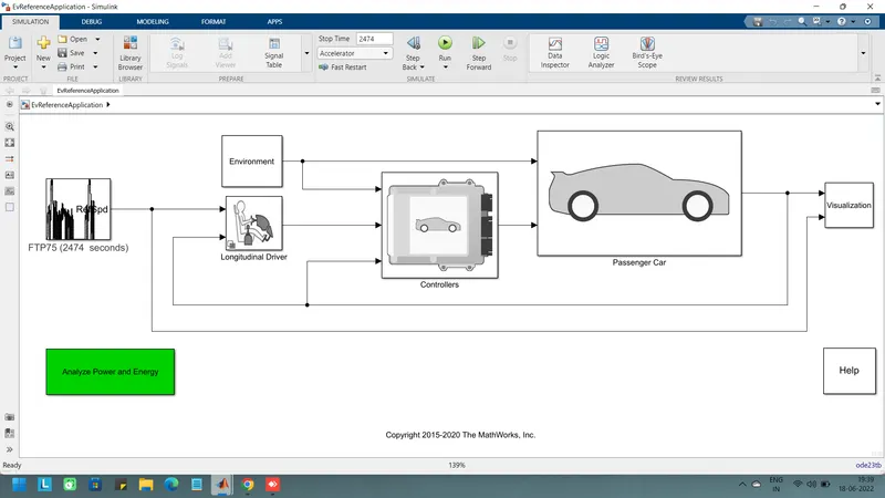
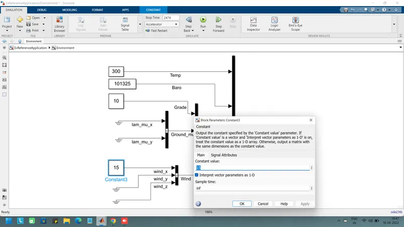
Then changing the FTP drive cycle to WOT drive cycle by clicking the block parameters of drive cycle.

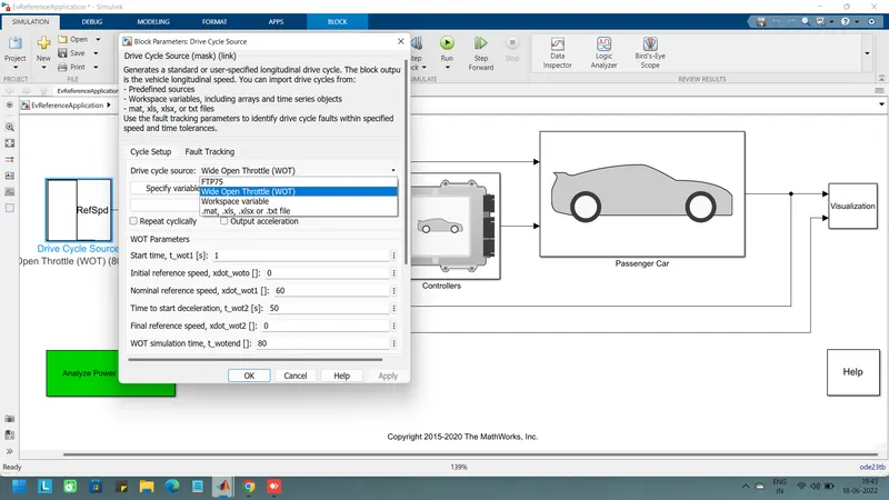
Changing the grade and wind velocity in the environment block remaining all parameters as default.

The grade angle=10 degree

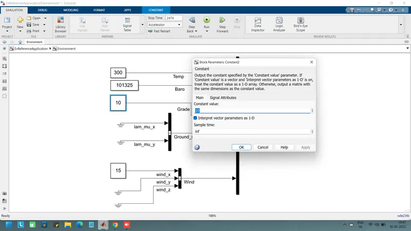
The wind velocity =15 m/s

Results:

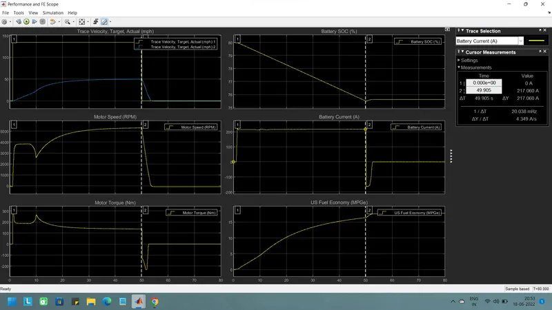
The above results shows results of the simulation and it consists of six plots.

Coursor measurement is helps in reading results in better way.

Plot 1: Trace velocity, Target & Actual(mph)

It shows the velocity of the drive cycle data with the time scale on x-axis.

top speed achived=50 mph

The accceleration time to reach the 50 mph = 49.9 sec

the decceleration time from 59.5 mph to minimum =4.24 sec

Plot 2: Motor speed

It shows the changes in the speed of the motor rpm through out the drive cycle.

peak motor speed =5010 rpm

Plot 3: Motor torque

It shows the changes in the torque of the motor in rpm through out the drive cycle.

peak motor torque =129 nm

A negative torue is seen after 30 sec it is due to regenerative braking.

Plot 4 :Battery SOC

It shows the battery state of charge SOC(%) and its changes corresponding to the driving inputs.

The state of charge decreased from 80% to 75.5% of charge in 49.71 sec ,for the specified driving conditions.

Plot 5 : Battery current(A)

It shows the battery current values (A) and its changes for various acceleration inputs as per the drive cycle.

The peak current discharge from the battery = 217A

The peak current charging to the battery = -162A

A negative battery current value indicates regenerative braking.

Plot 6: US fuel economy MPGe

It shows the fuel economy as miles per gallons for the corresponding input driving conditions.

Comparision and conclusion of pure ev and hybrid vehicle with same condition.

1.In a full electric vehicle achives a less top speed as compared to hybrid vehicle.

2.Battery discharging capacity is more in pure ev beacuse of lithium -ion battery is used as compared to hybrid vehicle.

3.Efficiency of the electic vehicle is higher than that of hybrid .

4. Electric vehicle produces zero emissions where as the hybrid one produce waste gas emissions