WOT Condition

Aim:

To study about the powertrain block set which includes full EV reference and HEV reference applications. We will also be changing the parameters and also studying how the basic calculations are performed.

Objective:

1. What is the difference between mapped and dynamic model of engine, motor and generator? How can you change model type?
2. How does the model calculate miles per gallon? Which factors are considered to model fuel flow?
3. Run the HEV Reference Application with WOT drive cycle. Change the grade and wind velocity in the environment block. Comment on the results.
4. Keeping all other parameters same, compare the simulated results of hybrid and pure electric powertrains.

Theory:

Wide Open Throttle (WOT)

Wide open throttle (WOT) refers to an internal combustion engine's maximum intake of air and fuel that occurs when the throttle plates inside the carburettor or throttle body are "wide open", providing the least resistance to the incoming air.[1] In the case of an automobile, WOT is when the accelerator is depressed fully, sometimes referred to as "flooring it."

In the case of a diesel engine, which does not have a throttle valve, WOT is the point at which the maximum amount of fuel is being injected relative to the amount of air pumped by the engine, generally in order to bring the fuel-air mixture up to the stoichiometric point. If any more fuel were to be injected then black smoke would result.

At wide open throttle, manifold vacuum decreases. The higher manifold pressure in turn allows more air to enter the combustion cylinders, and thus additional fuel is required to balance the combustion reaction. The additional air and fuel reacting together produce more power.

Model 1:

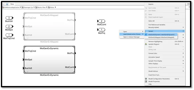
Difference between mapped and dynamic model of engine, motor and generator:

Mapped model of engine, motor and generator represent macro behaviour as a set of lookup tables (motor speed, power torque, brake torque, air mass flow, fuel flow, exhaust temperature, efficiency and emissions). In these tables we already have assigned values as it has a real time block i.e. a mapped motor lookup table in this can map the available motor data.

Dynamic model of engine, motor and generator is an actual model that shows the real components in which it is manually fed and has samples rates less than 1 second. Power electronics simulations are mostly performed dynamically. It is used to perform subsystem transient simulation for more detailed experiment i.e. in this we have actual PM controller and 3 phase voltage source inverter.

The mapped model takes less time than dynamic as it is less detailed and has a working range of 1 second.

Changing of model type:

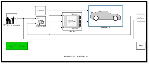
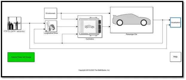
To change the model type we must enter into the corresponding block and then we must double click on the passenger car block.

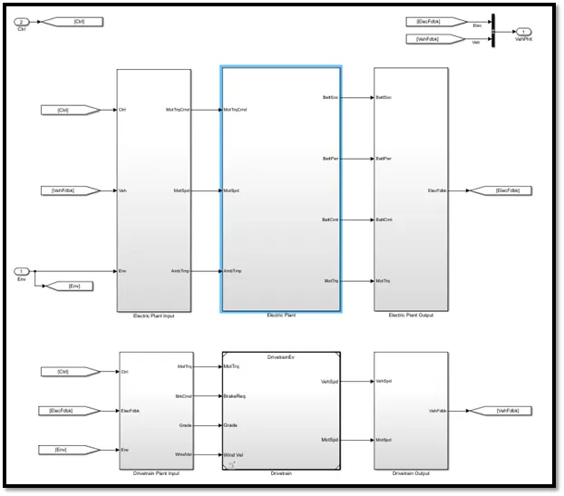
After which we must double click on the electric plant block.

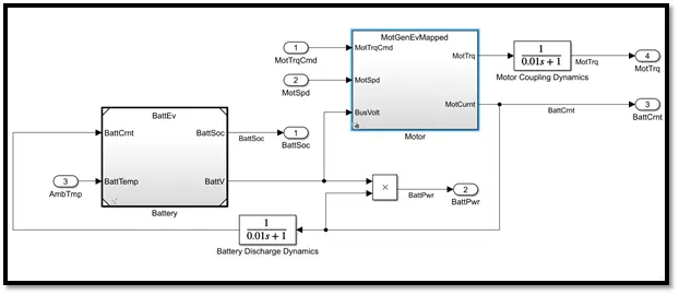
Then we must double click on the motor block.

We can now change the type from mapped to dynamic by right clicking on the empty place of the workspace ----> Variant -----> Label Motor Active Choice and then we can see that the type which is active is mapped and the same is also activated in our workspace.

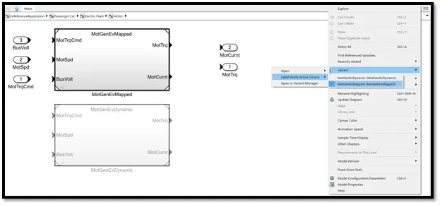
We can just change the type to dynamic and now we can see that the same is also activated in our workspace.

Model 2:

In order to study about how the model calculates the miles per gallon, we must first enter the corresponding block which is done by first clicking the visualization block.

And then entering the performance calculations block we can see the detailed calculations.

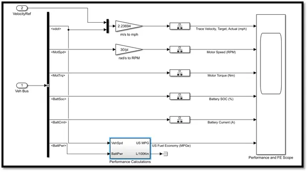
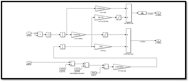
This calculation of battery power and vehicle speed in miles per gallon is used to find out how economical the battery is as compared to the fuel consumption. The vehicle speed and battery power are input to compare the fuel economy of engine to battery, the vehicle speed is converted to miles and battery power is converted to gallon using the following steps:

meter/second -----> product and square root -----> meter -----> bypass to next block -----> miles

battery power -----> divide by 1000 -----> kW -----> divide by 33.7 -----> gal/hr -----> m³/gallon

After that, the miles and gallon -----> product block -----> miles/gallon

Factors considered to model fuel flow:

1. Weight: The weight of the vehicle is considered as it plays an important role in determining the amount of fuel consumed as the weight increases the tractive effort required to overcome the vehicle’s rest inertia will increase.
2. Drive Cycle: At certain speeds the engine is able to operate at an rpm which provides maximum efficiency, driving at an irregular pace or higher speed makes the engine to provide lower efficiency. Aggressive acceleration and braking drive cycle decrease the fuel economy of the drivetrain.
3. Resistance: If the vehicle is subjected to high opposing wind speeds, road grade then there are high forces acting on the body, in particular, aerodynamic force and hill-climbing force. These forces increase the power needed to overcome the tractive effort, in turn making the engine consume more fuel. The effect of these forces can be reduced to a certain effect by making the vehicle more aerodynamic and light weight.

Model 3:

In order to run the HEV Reference Application using the WOT drive cycle we must select the drive cycle source in the model.

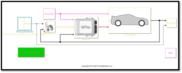
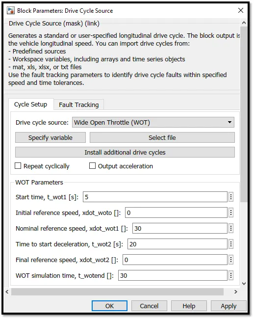
After which a new window will open and we can change the drive cycle source from the default one to the WOT and change some parameters like nominal reference speed and the WOT simulation time.

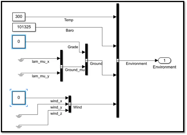
Then we must the change the grade and wind velocity before running the simulation. In order to do so we must double click on the environment block and then change the input values of grade and wind velocity in their respective constant blocks as shown in the figure below.

After we change the drive cycle and the values of the grade and wind velocity, we can run the simulation.

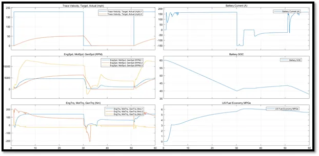
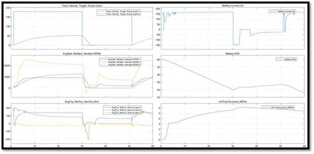
The vehicle velocity is less than the reference velocity as the grade and wind velocity have their impact. The maximum velocity obtained is 50 mph.

In this period the engine/motor/generator speed is around 13000 rpm which comes near to zero during regenerative braking. The maximum torque produced is 200 nm.

In initial 30 seconds the SOC declines its lowest up-to 42% and the battery current is about 160 A in this period.

The maximum fuel economy is about 6 mile per gallon at 32 seconds.

Model 4:

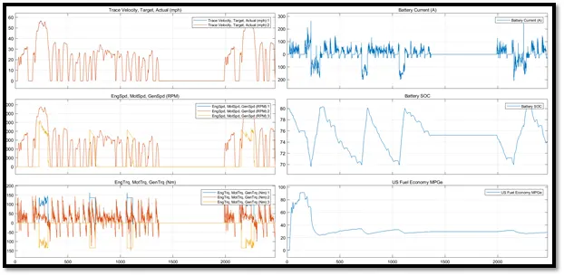
Initially we can run the simulation for HEV reference application without changing the drive cycle source and the environment parameters and results for the model is shown in the figure below.

Comparison:

Now we must set the conditions for the HEV reference application as WOT drive cycle source and change the grade and wind velocity values in the environment block. After we run the simulation, we can get the results plotted as shown in the figure below.

Now we must set the conditions for the EV reference application as WOT drive cycle source and change the grade and wind velocity values in the environment block. After we run the simulation, we can get the results plotted as shown in the figure below.

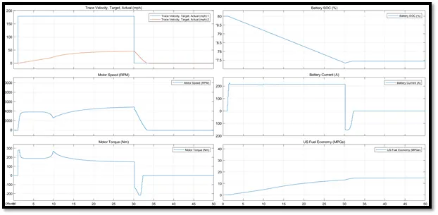
By comparing the plots of HEV and EV reference application, we can see that the maximum vehicle speed of HEV is higher than EV. The fuel economy of EV is very much higher than that of HEV. The EV SOC is at 77.5 % after 50 seconds while the HEV SOC is decreased from 60 % to 42 % after 50 seconds which makes the EV better than HEV. Torque and speed are higher in HEV than EV.

Conclusion:

1. The difference between mapped and dynamic mode was discussed and the steps to changed the model type was discussed.
2. The calculation of vehicle speed and battery to miles per gallon was explained and the factors considered to model fuel flow was discussed.
3. The HEV reference application was simulated by changing the drive cycle source and changing the parameters of grade and wind velocity and the plots were discussed.
4. Comparison was done for the change HEV and EV reference application and the plots were discussed.