Week-4 Challenge WOT Condition Part-2
Introduction to Hybrid E;ectric Vehicle using Matlab and Simulink
Challenge-4
Challenge WOT Condition Part-2
- What is the difference between Mapped and dynamic model of engine, motor and generator? How can you change the model type?
Objective:
To give a difference between mapped and dynamic model of engine, motor and generator and also how to change model type.
Power train Blockset:
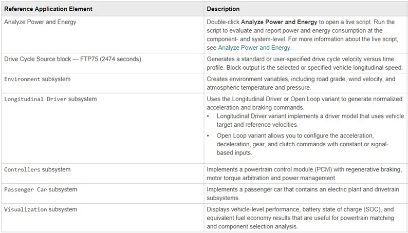
Power train Blockset provides fully assembled reference application models of automotive powertrain, including gasoline, diesel, hybrid and electric systems. It includes a component library for simulating engine subsystems, transmission assemblies, traction motors, battery packs and controller models.
Powertrain Blockset also includes a dynamometer model for virtual testing. MDF file support provides a standards-based interface to calibration tools for data import.
Powertrain Blockset provides a standard model architecture that can be reused throughout the development process. You can use it for design tradeoff analysis and component resizing, control parameter optimization and hardware-in-the loop testing. You can customise models by parameterizing components in a reference application with your own data or by replacing a subsystem with your own model.
Theory:
Difference between mapped and dynamic model of engine, motor and generator.
Engine - Mapped Model
Mapped engine models are suitable for analysis and design activities that do not require engine subsystem dynamic characteristics, for example in engine and transmission powertrain matching analysis for fuel economy, emissions and performance tradeoffs.
Engine – Dynamic Model
Dynamic engine models are suitable for designing control, estimator and diagnostic algorithms that depend on dynamic subsystems states for example in closed – loop AFR control algorithm development.
Motor – Mapped Model
The mapped motor block implements a mapped motor and drive electronics operating in torque – control mode. The output torque tracks the torque reference demand and includes a motor response and drive – response time constant. Use the block for fast systems-level simulations when you do not know detailed motor parameters, for example motor power and torque tradeoff studies. The block assumes that the speed fluctuations due to mechanical load do not affect the motor torque tracking.
Motor – Dynamic Model
The dynamic motor model use a real time or instantaneous values of the motor power and torque values by the running behaviour of the motor speed.
Generator – Mapped Model
The mapped generator model or blockset take lookup table power values from engine and saturate that values as for giving output to motors or change the battery capacity.
Generator – Dynamic Model
The dynamic generator blockset take instantaneous power output values from the engine and gives to the transmission or it use that power to charge the battery.
Steps to be taken to change the model type in powertrain blockset model /example reference model :
- Open and explore the EV reference application from getting started to powertrain blockset link, you will see EV model which contains environmental block, longitudinal driver, controller block, passenger car block, FTP75 drive cycle Block etc.
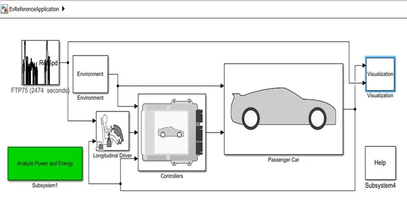
2. Open the passenger car block by double click on it, after its opening you can see there many other blocks such as electric plant, drivetrain block, electric input-output block etc. 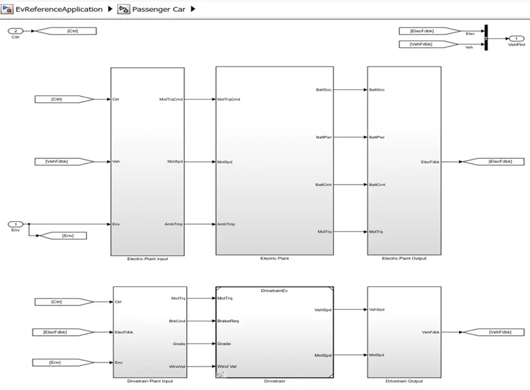
3. Open the electric plant block then you can see other different blocks of motor and battery packs.
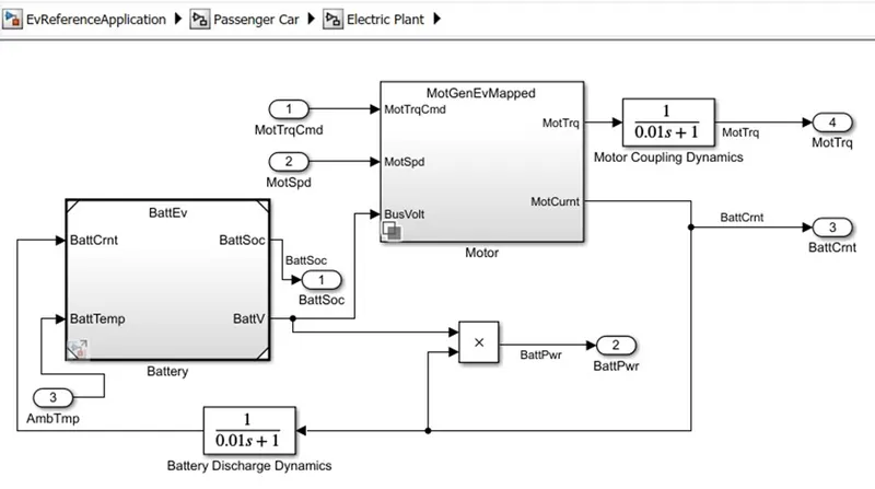
4. Open the motorgenEVmapped block, you can see there are two blocks available for switching which are
1.motorgenEVmapped block
2.motorgenEVdynamic block
and in which motorgenEVmapped block is by default selected.
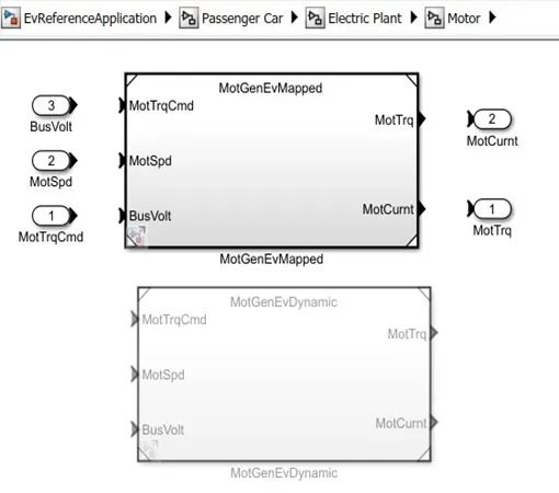
5. For changing variant, right click on screen select the variants option from the list of options available in that you will get another options select to label mode active choice there you can change from mapped EV model to dynamic EV model.
- How does the model calculate miles per gallon? Which factors are considered to build model fuel flow?
Miles per gallon (MPG) is a fuel economy rating determined by how far a car or any vehicle can travel on a gallon of gasoline or diesel. Although the metric would be also kilometres per litre, MPG is adopted in many metric-system countries.
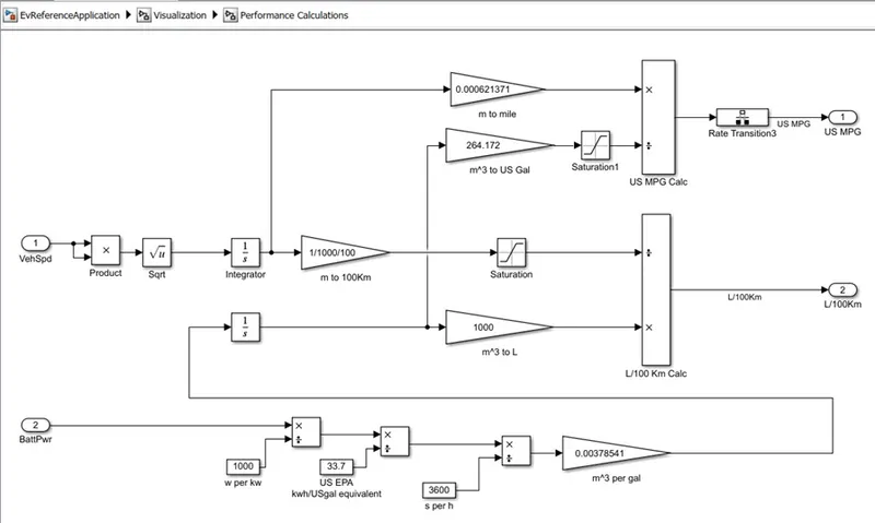
In this EV model derived or opened above had a visualisation block where we can get the idea that how we get the value for MPG (miles per galon) which is also seen in the below block diagram arrangement.
Block Diagram:
EV Reference Application Model:
Model Calculation:
- The battery power is taken in watt (W) and then divided by 1000 to convert into KW.
- Then the resultant power in KW is divided by 33.7 (KWh/US gal)(constant US EPA value).
- The (US gal/h) value is converted into (US gal/sec) by being divided by 3600.
- The value is then multiplied by 0.00378541 to convert into (m^3/gallon).
- This value is taken and then integrated so that we obtain it in (m^3).
- Besides that, the vehicle speed is taken and then squared then square root is taken in order to remove the negative values then integrated to obtain speed(in m).
- The speed (m) value is multiplied with 0.000621371 to convert it from metres to miles and then integrated (m^3/gallon) value is divide with (264.172) to convert it into m^3 to US gallon and pass this value from saturation block to obtain saturated speed value in milers per gallon(MPG).
- As this is an EV reference application model/ pure electric vehicle model so it is fully dependent on battery source and there is no need of fuel flow data.
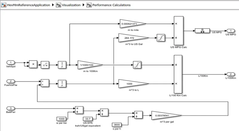
HEV Reference Application Model:
Model Calculation :
- As step 1 to 4 is continued as well as mentioned in the above block diagram for EV Reference application.
- This value is taken in m^3 per gallon is then added with fuel volume flow value and then integrated so that we obtain it in (m^3) value.
- Rest from Step 6 and 7 is continued as well as mentioned for above block diagram.
- As this is an HEV reference application model so not only dependent on battery source as there is also fuel flow data provided as secondary source.
- Run the HEV Reference Application with WOT drive cycle. Change the grade and wind velocity in the environment block. Comment on the results.
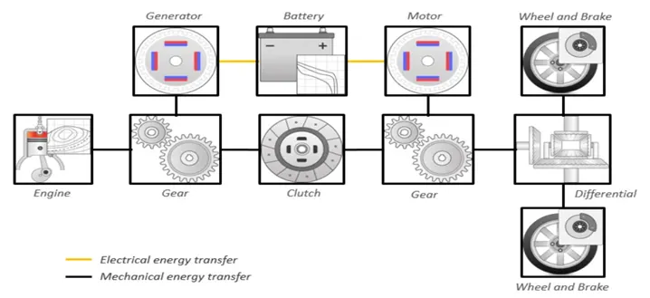
Solution: Components used in Hybrid Electric Vehicle (HEV) powertrain are as follows:
- Engine
- Gearbox
- Generator
- Battery pack
- Clutch
- Motor
- Differential
- Wheels and Brake
Simulink Model
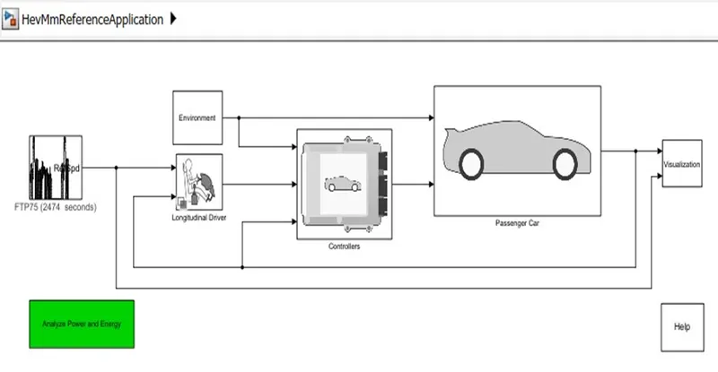
In the model you can see that there are several numbers of blocks or subsystems named with Controllers, Environment, Passenger car, Longitudinal Driver, FTTP75 Driver Cycle block, Visualisation block.
- Controller block consists consist of power control module(PCM) which is master control of the vehicle, it contains Engine Control Module (ECM) and Hybrid Control Module (HCM) which will control motor and battery management system, it will control the power supply as combination of series and parallel or series alone or parallel alone.
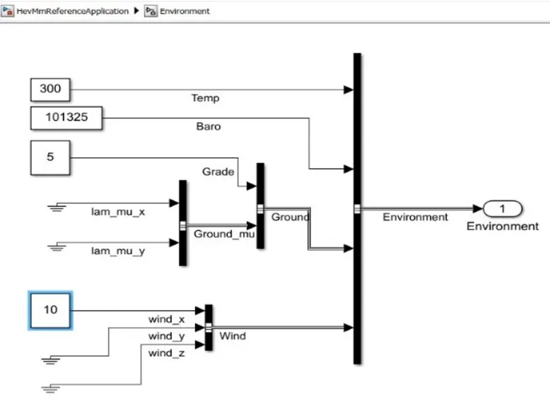
- Environment block gives the idea of physical environmental conditions (wind velocity, grade value, temperature and pressure) which will be acting on the vehicle in motion.
- Passenger car block consists of various sub blocks which are engine block, engine plant block, drivetrain block. Its whole like an actual transmission block. Engine block will be containing mapped and dynamic models are there to function as per the driving conditions. Engine plant block contains sub blocks of battery, generator and motor blocks which will control the behaviour of battery, generator and motor respectively.
- Longitudinal driver block contains all the driver related parameters which he will be supplying throttle gear change, braking motion all are controlled in it.
- FTP75 block is predefined drive cycle block which gives the drive cycle as per the default values given to it. We can change this block with our own input values of speed variations as per the road conditions.
- Analyse power and Energy blocks used there is so that we can solve the whole parameters and can get the output in a tabular form. We can get run summary, electric plant summary, drivetrain summary, overall summary.
Simulink Result : Performance PE Scope (with FTP drive cycle) :
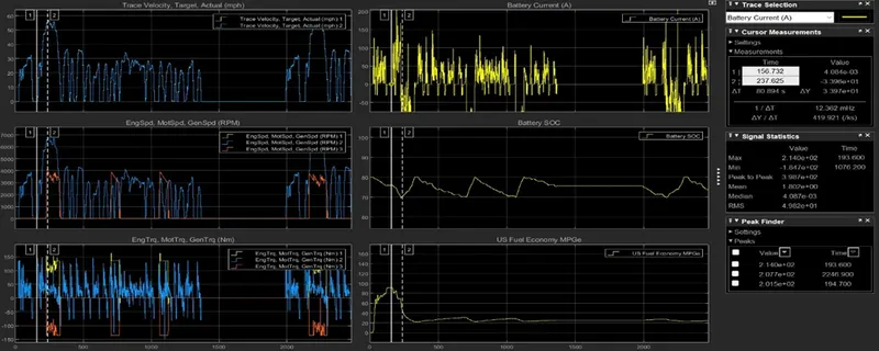
So, this is the performance PE graph of HEV with FTP drive cycle run under 2475 stop time seconds. In this graph you can see and understand that how each and every plot relate to other one.
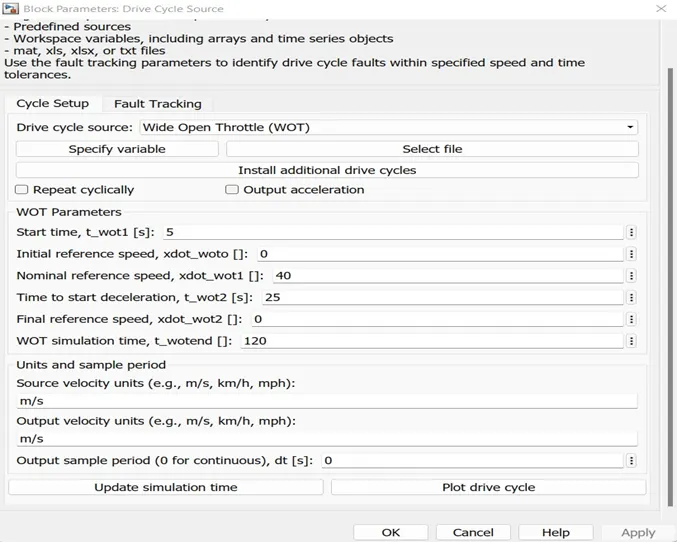
Now, Change this drive cycle from FTP75 to WOT drive cycle to check the variation in output in the form of traces in the scope and run this drive cycle for 120 seconds.
Simulink Result : Performance PF Scope ( with WOT drive cycle) :
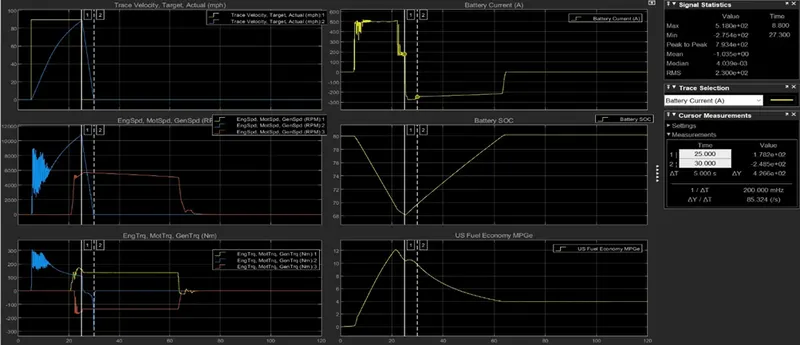
In this plot graph you can see that there are different traces plotted here for indicating 6 different parameters and their conditions. So let see what I understand from these graph:
- In the first velocity plot graph yellow line indicating for WOT input data given to model and blue line indicating the output data of velocity provided by the model. Now, I understand that resultant it starts from 0 m/s at 5 sec and it goes upto 89.5 m/h and then deaccelerating for 5 sec (from 25 to 30 = 5 sec) to reach to 0 m/h.
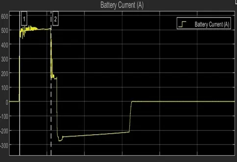
- In second battery current plot graph there is only single yellow line indicating battery current having variation according to output resultant velocity of the model. It consume or utilise the current in just 22 seconds (after 17 sec of acceleration) and then reduces its strength of consumption as vehicle starts deaccelerating.
- In third plot graph there are 3 different parameters of speed indicating yellow for engine, blue for motor and red for generator. So engine and generator speed action takes place at the same time from 20 sec and both continues as the vehicle deaccelerating and motor takes action when just vehicle accelerating from 5 sec and there is a glitch action graph (as you can see in the graph as well) to 12 or 13 seconds ( for 7-8 seconds) because the vehicle suddenly start with speed of 0 m/s and its start within its nominal reference speed is 40 m/h and then increases gradually with linear speed.
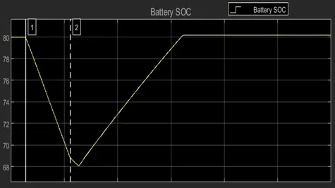
- The fourth plot graph is for battery SOC which indicates that how much battery is consumed here (as this is a HEV so it is not fully dependent on this). But as the vehicle starts at 5 sec and accelerate till 25 sec, it consumes 14.76% of SOC. When vehicle starts deaccelerating the battery regaining its SOC and it rises up gradually to 64 seconds(took 39 sec from it starts deaccelerating) till getting its original battery SOC value.
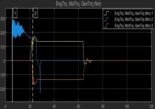
- The fifth plot graph is for torque management of three different parameters indicating yellow for engine, blue motor and red for generator. So, here Engine and generator action takes place simultaneously but in opposite direction and motor keep in action from vehicle just begin to accelerate and it again shows some glitches type graph (as you can see in the graph above) to 17 sec (for 12 sec) and then rises with linear motion with follow-up the engine speed characteristics.
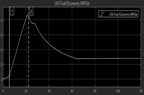
- The sixth plot graph is for US fuel economy which gives the idea of how much fuel is consumed by vehicle and what is the economy of it under US rules. Now, when vehicle just start accelerating it starts from 0 (zero) and then increases gradually for the time interval of 20 sec (from 0 to 20 sec) and then starts falling its value till 63 sec time interval and then its value is uniform to 3.99 (approx.. 4.0).
With this WOT drive cycle if the grade value and wind values is changed from environment block as you can see below image attached here make some changes which I got after simulating the model for stop time 120 sec.
Environment Block :
Simulink Result : Performance PE Scope ( after change in grade and wind value) :
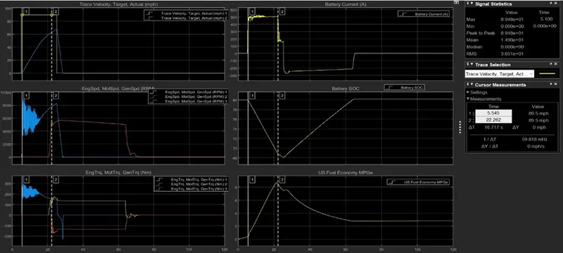
- In WOT if the grade value and wind values is changed then there is change in velocity trace the linearity attained is 67.1 mph of top speed is attained at 25 sec of time. Till 32 sec speed is been increasing slowly and then decreasing to 28 sec to reach its initial value 0 mph.
- Remaining all other graphs plotted of battery SOC, battery current, speed, torque and fuel economy looks same.
4. Keeping all other parameters same, compare the simulated results of hybrid and pure electric powertrains.
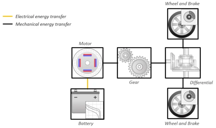
The components in hybrid Electric Vehicle (HEV) powertrain are as follows,
- Gearbox
- Battery pack
- Motor
- Differential
- Wheel and Brake
EV Model power train Configuration :
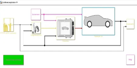
EV reference Application :
Simulink Result : Performance PE Scope (with FTP drive cycle) :
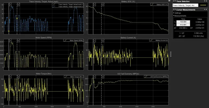
So, this is the performance PE graph of EV with FTP drive cycle run under 2475 stop time seconds. In this graph you can see and understand that how each and every plot relate to other one.
Now, Change this drive cycle from FTP75 to WOT drive cycle to check the variation in output in the form of traces in the scope and run this drive cycle for 120 seconds.
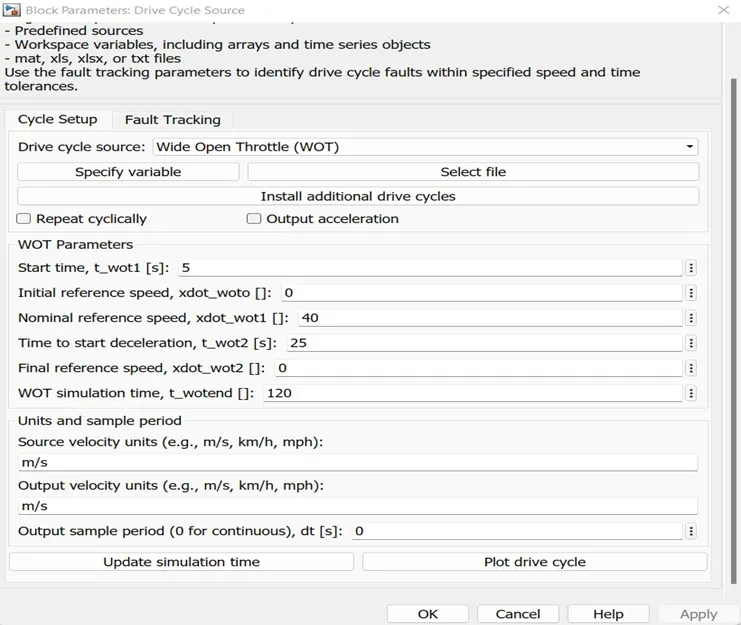
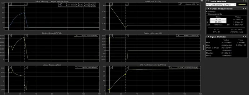
Simulink Result : Performance PE Scope (with WOT drive cycle) :
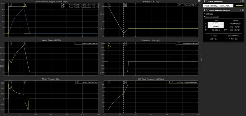
In this plot graph you can see that there are different traces plotted here for indicating 6 different parameters and their conditions. So let see what I understand from these graph :
- In the first velocity plot graph yellow line indicating for WOT input data given to model and blue line indicating the output data of velocity provided by the model. Now, I understand that the data given through drive cycle goes upto 89.5 mph from time interval of 5 to 25 sec and the resultant it starts from 0 mph at 5 sec and it goes upto 81.92 mph and then deaccelerating for 5 sec (from 25 to 32 sec = 7sec) to reach to 0 m/h.
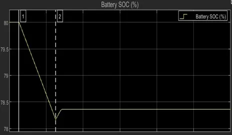
- The fourth plot graph is for battery SOC which indicates that how much battery is consumed here (as this is an EV so it is fully dependent on battery pack) and initially battery SOC is at 80 %. But as the vehicle starts at 5 sec and accelerate till 25 sec, it consumes 2.287% of SOC and reaches to 78.18%. Then vehicle starts deaccelerating so the battery regaining its SOC and it rises up gradually to 30 seconds (took 5 sec from it starts deaccelerating point) till getting its linear battery SOC to 78.48 %.
- In third plot graph there is only one parameters of speed indicating yellow for motor (as this is an EV Model, there is no need of engine and generator).So motor only takes action when just vehicle accelerating from 5 sec and there is a sudden action graph (as you can see in the graph as well) to 8.6 or 8.7 seconds (for 3.6 – 3.7 seconds) because the vehicle suddenly start with speed of 0 m/s and its start within its nominal reference speed in 40 m/s and then increases gradually with linear speed for time period of 25 sec and then as vehicle deaccelerating so the motor’s graph starts falling down to zero.
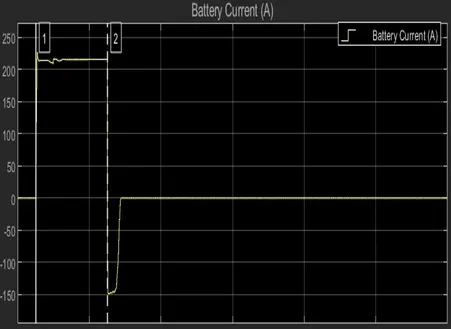
- In second battery current plot graph there is only single yellow line indicating battery current having variation according to output data of velocity of the model. It consumes or utilise the current for full acceleration time period from 5 to 25 seconds (for 20 sec). Initially, In the graph you found some glitches because of sudden action of vehicle from very zero inertia then there is a linear consumption of current and then reduces its strength of consumption as vehicle starts deaccelerating comes to finally zero (as you can see in the graph).
- The fifth plot graph is for torque management indicating yellow for motor. So, motor keep in action from vehicle just begin to accelerate in 5.12 sec and it goes upto torque value 273.467 N-m and it again shows some small glitch type graph to hold linear torque (as you can see in the graph above). It takes 3.375 sec having torque 249.198 N-m and then falling with linear motion to deaccelerating point of 25 sec and then reach to a -ve torque value of 71.289 N-m. It again fall to 30 sec (final deacceleration point) and have torque -208.783 N-m and then reach to zero.
- The sixth plot graph is for US fuel economy which gives the idea of how much fuel is consumed by vehicle and what is the economy of it under US rules. Now, when vehicle just start accelerating it starts from 0 (zero) and then increases gradually for the time interval of 20 sec (from 0 to 25 sec) and while deacceleration its value have a sudden boom and reach to a value of 3.49 then it becomes straight linear with constant value 3.51.
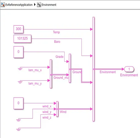
With this WOT drive cycle if the grade value and wind values is changed from environment block as you can see below image attached here make some changes which I got after simulating the model for stop time 120 sec.
Environment Block :
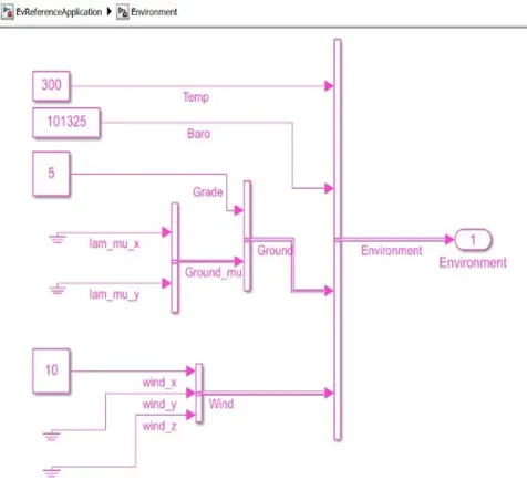
Simulink Result : Performance PE Scope (after change in grade and wind value) :
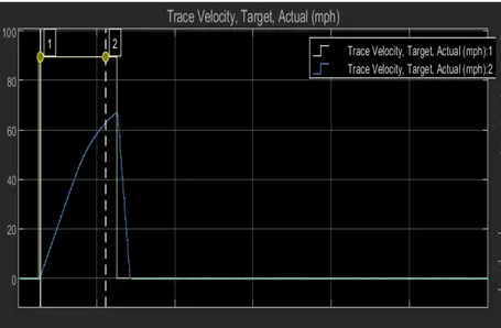
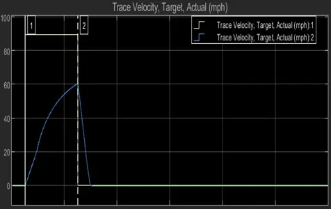
- In WOT if the grade value and wind values is changed (as you can see in the above fig. ) then there is change in velocity trace.The linearity attained by the velocity-2 is 60.4 mps which is a top speed and is attained at just 20 sec of time interval. Till 25 sec speed is been increasing slowly and while deaccelerating it is decreasing to 30.0995 sec to reach its approx. initial value 0 mps.
- Remaining all other graphs plotted of battery SOC, battery current, speed, torque and fuel economy looks same.
Comparison between EV & HEV : Simulation output :
1. If we compare velocity trace plot of EV reference to HEV reference for attending maximum velocity, EV vehicle takes more time as compared to HEV.
EV_Reference_Model HEV_Reference_Model
2. EV vehicle consumes about 60% of battery SOC more than HEV because EV is a pure electric vehicle and fully dependent on battery pack but HEV is not only dependent onlu on battery but had fuel source too.
EV_Reference_Model HEV_Reference_Model
3. EV vehicle consumes 30-40% more current than HEV.
EV_Reference_Model HEV_Reference_Model
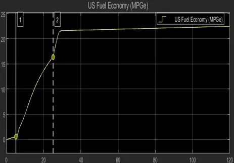
4. Miles per gallon of EV is 21.13% and for HEV, its was 10%.
EV_Reference_Model HEV_Reference_Model
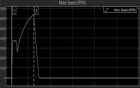
5. Motor torque is almost same in both the cases.
EV_Reference_Model HEV_Reference_Model