Week-3 Challenge: ADVISOR Tool
Introduction to Hybrid Electric Vehicle using Matlab and Simulink
Challenge-3
1.Using EV_default_in file, if cargo mass is 500 kg with other default conditions. To find whether the vehicle can travel for 45 km with FTP drive cycle? And to conclude observations.
Answer:
Objective: To find whether the vehicle can travel for 45 km with FTP drive cycle using EV_default_in file from ADVISOR, if cargo mass is 500 kg with other default conditions.
Theory:
ADVISOR tool, developed in November 1994 by the National Renewable Energy Laboratory (NREL), allows users to simulate and analyse conventional, light and heavy vehicles, including hybrid electric and fuel cell vehicles. The tool allows users to assess the effect of changes in vehicle components (such as motors, batteries, catalytic converters, climate control systems and alternative fuels) and other modifications that might affect fuel economy, performance or emissions. In development point of view, it is being old or outdated but because of its high utility point of view, it is popular as well. Vehicle models are mostly experimental, relying on drivetrain components I/O relationship measured in the lab.
It is a set of models, data and scripts text files for use with Matlab and Simulink. The benefits of using ADVISOR tool:
- Estimate the fuel economy of vehicles/model that have not yet been built in reality.
- Help us to learn about how conventional, hybrid or electric vehicles uses (and loses) energy throughout their drivetrain.
- Compare relative tailpipe emissions produce on a number of cycles.
- Evaluate an energy management strategic for your hybrid vehicle’s fuel converter.
- Optimise the gear ratio in the transmission to minimise fuel use or maximise performance etc.
Take a look that how we can start ADVISOR tool.
- Launch MATLAB software and first set default location folder for the ADVISOR to load file/work.
- Now in the Matlab command window, type “ADVISOR” and press enter and wait until it load.
- A new window will open and then set “metric” as unit and start ADVISOR.
- It will launch in a new programmable or pre-designed window for simulation.
This ADVISOR tool window consists of 3 different windows where we understand, work, simulate with different inputs and get a variety of new outputs/results. ADVISOR tool particularly have 3 windows:
- Vehicle input window : In this window we can launch or can see or observe new vehicle models which is already designed here.
- Simulation parameter window : In this window we can change the parameters like of the gear ratio, no. of drive cycles, fuel converter type, mass of cargo etc.
- Results window : In this window we will get a kind of final result in the form of graphical interface which is also of our choice to see by changing the parameters. Here, we can also see some other important things like fuel consumption, gradeability etc.
Observation:
There is a default vehicle load file model which you can seen here in the below fig (1) which is PARALLEL_default_in with some default parameters which you can also see below in the Simulation Parameter window.
By clicking over the load file option having drop down menu and switch from the parallel_deafault_in to EV_default_in option.
Now, change the mass of cargo from 136 kg to 500 kg keeping all other parameters same as it is and there you can see the change in the total mass of the vehicle from 1350 kg to 1508 kg.
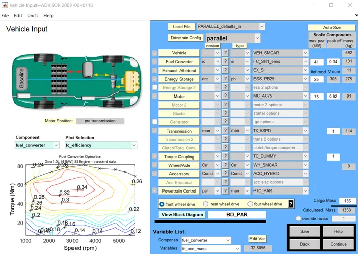
Fig 1: PARALLEL_default_in
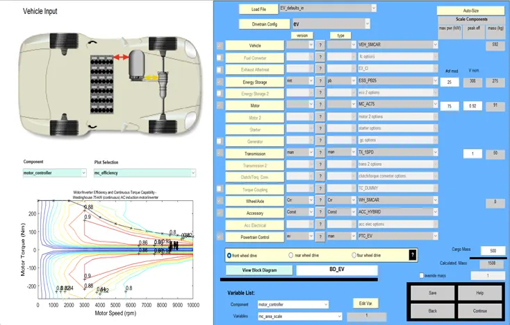
Fig 2: EV_default_in (with change in cargo mass)
Then, go to continue option as I have mentioned below in fig 3.
Fig 3: Go to continue
Here, you can see there is a drive cycle option having drop-down menu to change the drive cycle to CYC_FTP to check whether the vehicle can travel upto 45 km under the given drive cycle.
Here, you can also change the no. of drive cycle from # of cycle. But, now keep this value to 1 to check the output under the given drive cycle.
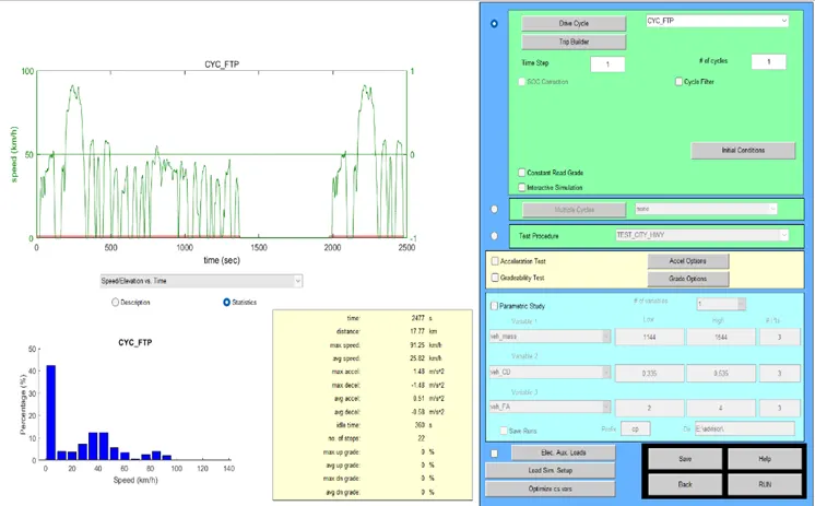
Fig 4: To change the drive cycle.
Go to run option available in the rectangular block as shown as highlighted in the fig 5 below.
Fig 5 : Go to run
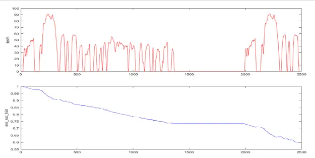
Fig 6: plot graph of distance travelled by vehicle and SOC.
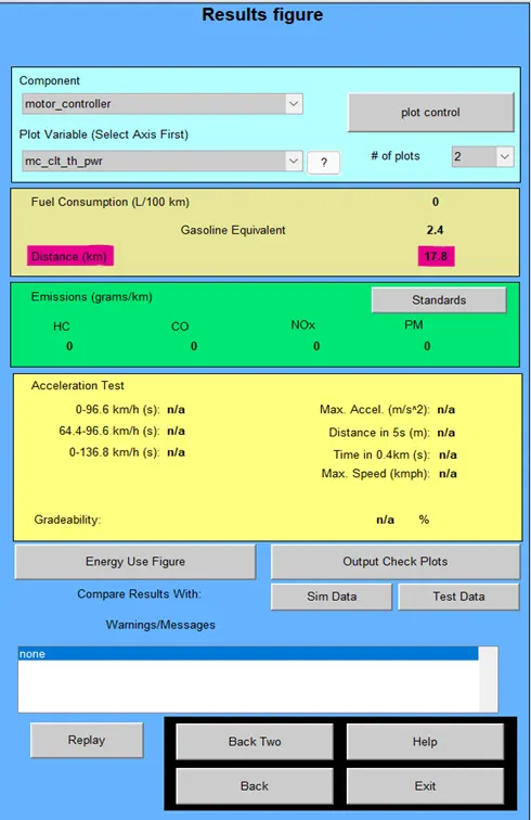
Fig 7: final output value
So, with 1 no. of drive cycle the vehicle could only travel upto 17.8 km. Therefore, I change the no. of drive cycle from 1 to 2 keeping all other parameters same.
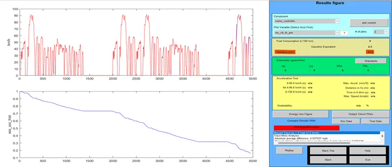
Fig 8: Output at drive cycle 2.
Again, the vehicle could only cover a distance upto 35.5 km which is not the requirement of the question. Therefore, change the no. of drive cycle from 2 to 3 and see the final output.
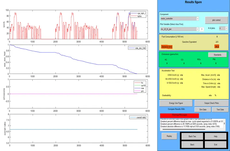
Fig 9: Output at drive cycle 3.
Again, it couldn’t reach to its required value as it is very close to it.
Conclusion:
From the above experiment in ADVISOR tool, I understood that every object have certain limit and capability to do. Here, in this case by changing the weight of cargo, the load of vehicle increases above to its limit and that’s why it was not able to perform well by changing the number of drive cycles keeping its source of energy same affects the driver of vehicle.
----------------------------------------------------------------------------------------------------------------------------------------------------------------------------------------------------------------
2.In the above case, try changing the battery capacity and repeat the simulation.
Answer:
Objective:
To find whether the vehicle can travel for 45 km with FTP drive cycle using EV_default_in file from ADVISOR, if cargo mass is 500 kg, make a change in battery capacity and keep all parameters same.
Observation:
To change the battery capacity, go to #of mod option available in right top of the vehicle input window (as shown in the fig 2).
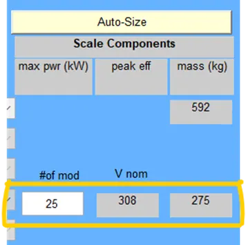
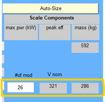
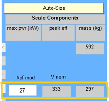
Fig 10 : with increasing the battery capacity , the weight of the vehicle also increases.
Here, you can see while changing the battery capacity value create a variation in voltage level and there is also change in the weight of vehicle.
As previously we have seen in this report, the output result in the fig 7, 8 and 9 with the battery capacity 25 and drive cycle no. 1, 2 and 3. It doesn’t satisfy the question requirement. Now, with increasing the value to 26 (keep it constant) and increase the no. of drive cycle to get the desired output.
Case 1 :
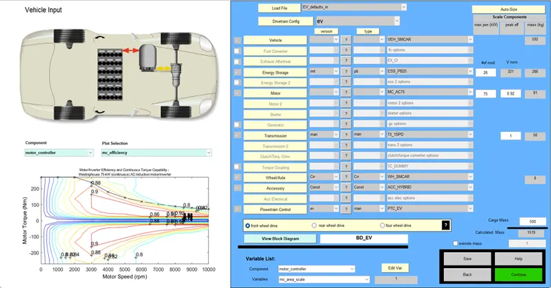
Fig 11: change the battery capacity and go to continue.
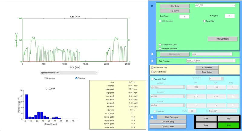
Fig 12: change the no. of drive cycle and go to run.
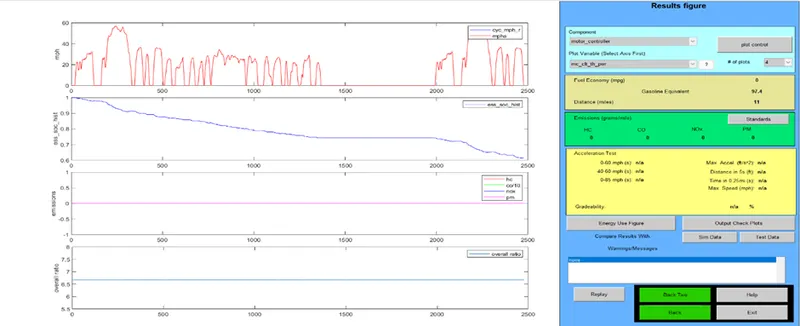
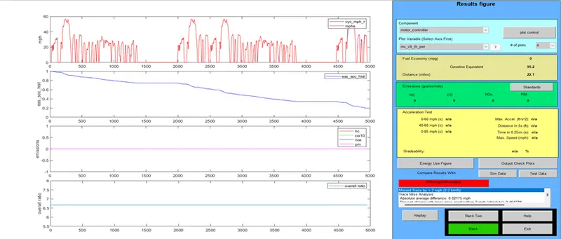
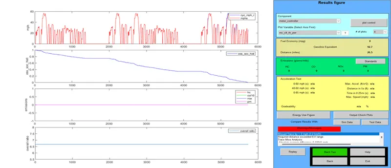
Fig 13. : Result for case 1 under battery capacity 26 and no. of cycle is 1, 2 and 3.
As previously we have seen the output result in the fig 13 with the battery capacity 26 and drive cycle no. 1, 2 and 3. It doesn’t satisfy the question requirement. Now, with increasing the value to 27 (keep it constant) and increase the no. of drive cycle to get the desired output.
Case 2 :
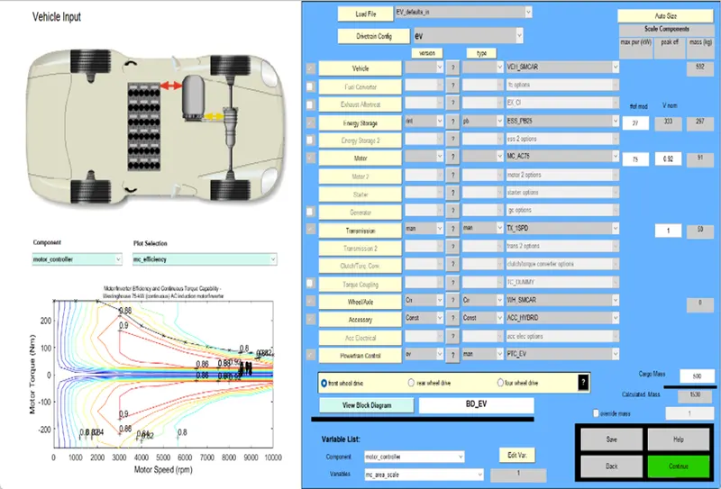
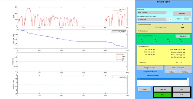
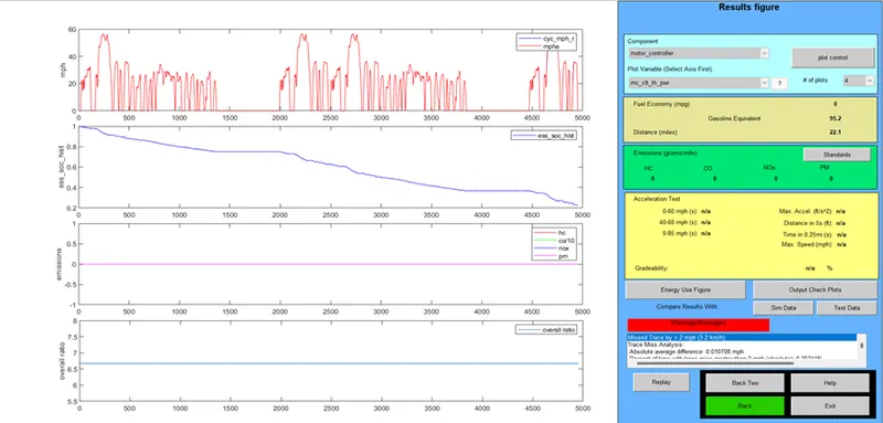
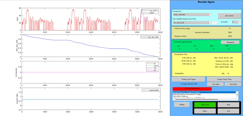
Fig 14.: Result for case 2 under battery capacity 27 and no. of cycle is 1, 2 and 3.
As previously we have seen the output result in the fig 14 with the battery capacity 27 and drive cycle no. 1, 2 and 3. It doesn’t satisfy the question requirement. Now, with increasing the value to 28 (keep it constant) and increase the no. of cycle to get the desired output.
Case 3:
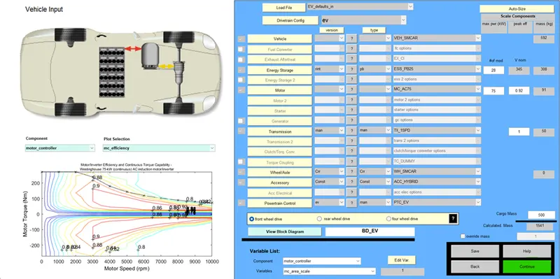
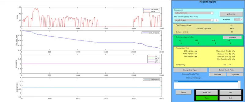
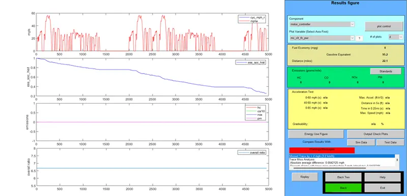
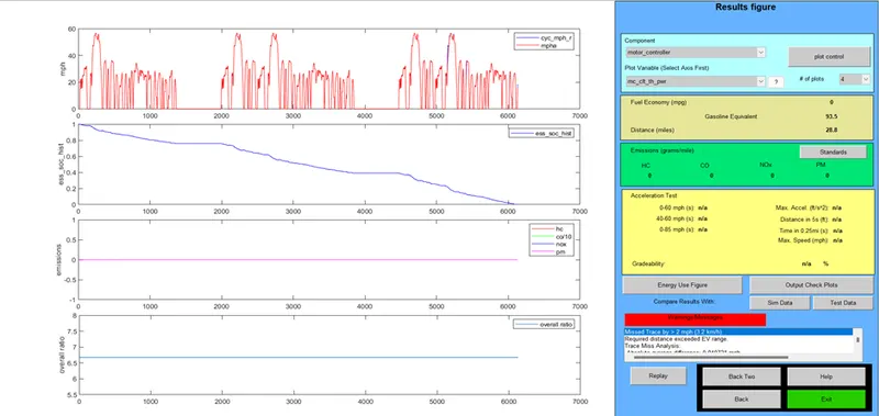
Fig 15.: Result for case 3 under battery capacity 28 and no. of cycle is 1, 2 and 3.
Conclusion:
Whatever I observe from fig 13, 14 and 15, you can understand from the given data available in table as I have mentioned below.
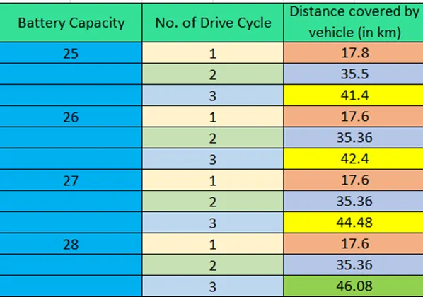
So, you can see here with any battery capacity either for 25 or 26 or 27 or 28 the distance covered by vehicle is upto same 17.6 km under drive cycle 1 and 35.6 km under drive cycle 2.
Again, for battery capacity 25, 26 and 27 the distance covered by vehicle is very close to the desired value but due to some warning (highlighted red in colour as shown in the fig 13, 14 & 15 )and inefficiency of SOC in each case it cannot exceed.
But, In case 3 with battery capacity 28 and no. of drive cycle 3, it was possible as you can see above in the table mentioned (highlighted in green colour).
-------------------------------------------------------------------------------------------------------------------------------------------------------------------------------------------------------------------
3.To perform gradeability test with PRIUS_Jpn_default_in file. To compare results in the table and conclude.
Objective:
To perform gradeability test with PRIUS_Jpn_default_in file. And compare there results in the table and make a conclusion of report.
Theory:
- First open ADVISOR and change the vehicle model from drop-down option and open PRIUS_Jpn_default_in file to work and for understanding the model.
- Now, without any change, click over the continue option.
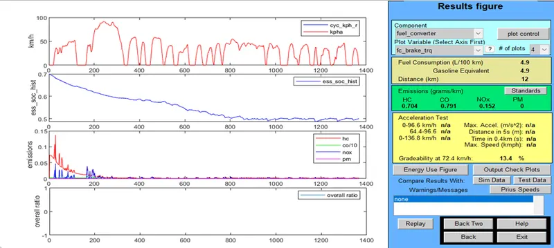
- Tick on Gradeability Test and click on Grade options and a new window will open where I change the the value of speed.(as shown in the fig16)
- Now, enable All system and Current mass (as shown in the fig17) and click OK.

Fig 16: gradeability test
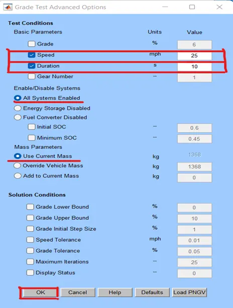
Fig 17: Gradeability advanced options
- Then, click on run button to get the result of gradeability test and note down the value of gradeability at the given speed.
- As described above steps do further more times at different speed and at different time interval and note down all the values in a table to get a final conclusion.
At time interval 10 sec.
At speed 25 m/h or 40.2 km/h.
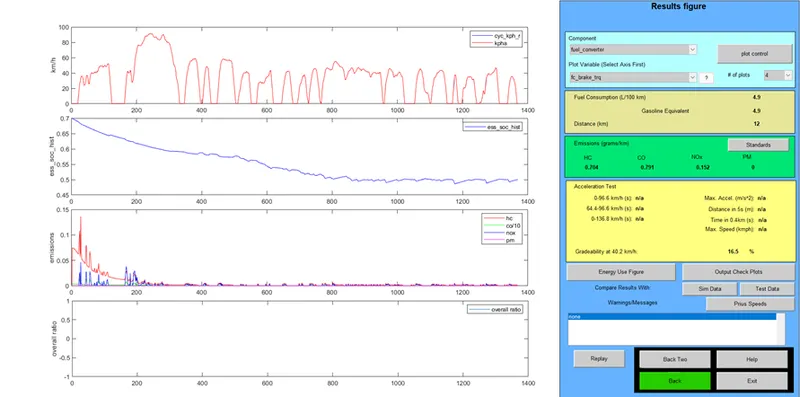
At speed 30 m/h or 40.2 km/h.
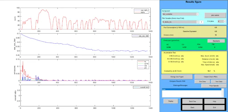
At speed 35 m/h or 56.3 km/h.
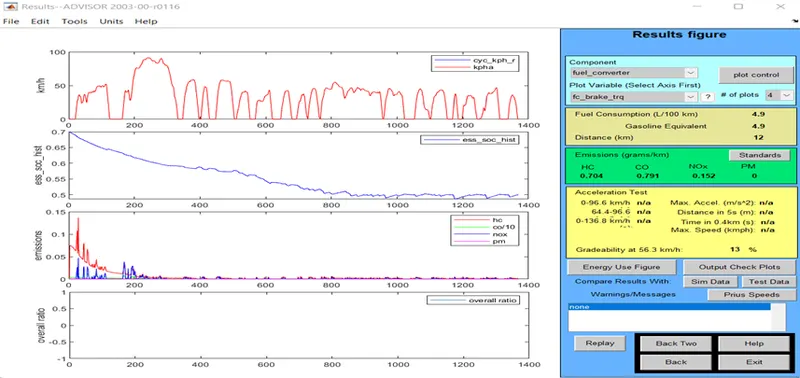
At speed 40 m/h or 64.4 km/h.
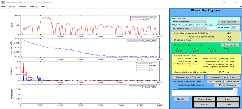
At speed 45 m/h or 72.4 km/h.
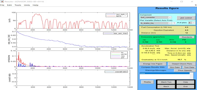
In time interval 20 seconds.
At speed 25 m/h or 40.2 km/h.
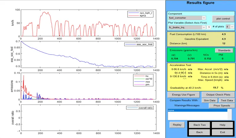
At speed 30 m/h or 40.2 km/h.
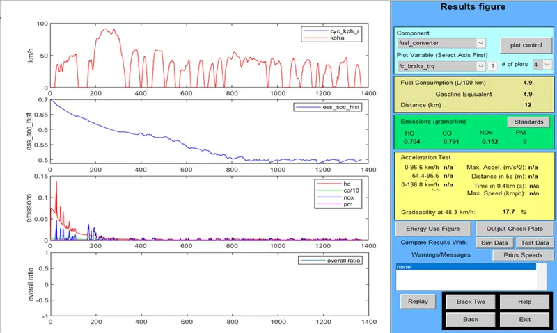
At speed 35 m/h or 56.3 km/h.
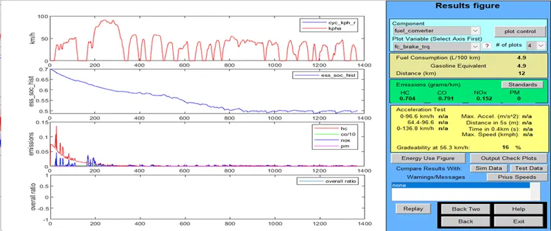
At speed 40 m/h or 64.4 km/h.
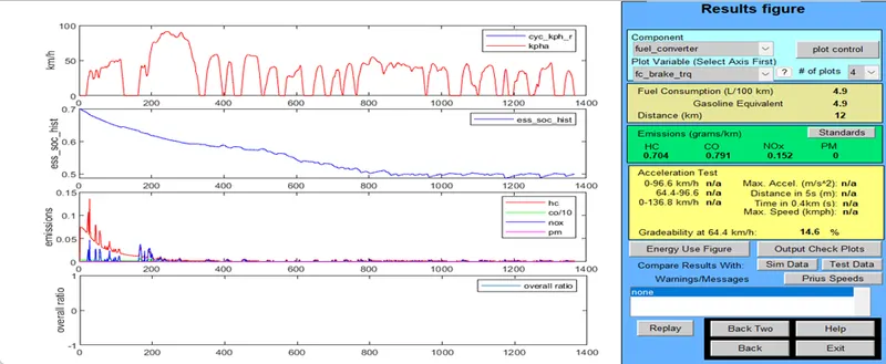
At speed 45 m/h or 72.4 km/h.
Conclusion:
After solving this model and checking gradeability test with variable speed at different time interval, I understood and observed that with rise in velocity the gradeability of the vehicle falls down or decreases at certain %.
I also made a table of gradeability test for this report, so it might be easy to understand this clearly.
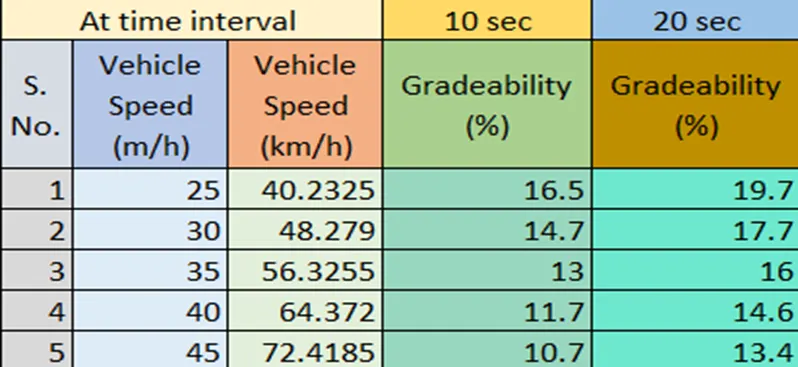
You can see here that I have taken 5 different test having vehicle speed 25, 30, 35, 40 & 45 m/h for each two different cases of time interval (10 & 20 sec).
And you can also see here and observe that gradeability of the vehicle decreases with increase in speed of the vehicle.