Week-4 Challenge WOT Condition Part-2

WEEK – 4

Q1. Difference between mapped and dynamic model of engine, motor and generator.

Powertrain Blockset provides two types of engine models: mapped and dynamic. Mapped engines represent macro engine behaviour as a set of lookup tables (brake torque, fuel flow, air mass flow, exhaust temperature, efficiency, and emissions) as function of commanded load and measured engines speed. Dynamic engines decompose engine behaviour into individual component models that account engines dynamics, most notably intake airflow and turbocharges dynamics. You can switch between engine model type based on your application. Dynamic engine models are suitable for designing control, estimator, and diagnostic algorithms that depend on dynamic system states, for example, in closed loop AFR control algorithm development. Mapped engine models are suitable for analysis and design activities that do not require engine subsystem dynamic characteristics, for example, in engine and transmission powertrain matching analysis for fuel economy, emissions, and performance trade-offs.

MAPPED MODEL:

• It uses a prebuilt data in lookup table for the simulation of powertrain block set.
• In mapped model the calculations are very fast.
• Electric losses are need to be specified if present.

DYNAMIC MODEL:

• It uses real time data for calculating every behaviour of vehicle characteristic like speed, vehicle, drag, wheel braking etc…
• In dynamic model the calculations are time consuming.

CHANGING THE MODEL TYPE:

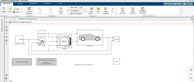
• Open EV reference application in the powertrain block set of MATLAB. It is a Simulink model which consist of drive cycle. Environment conditions, longitudinal driver controllers and passenger car.

• Now open the passenger car block and select the electric plant

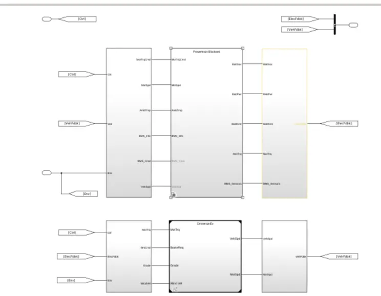
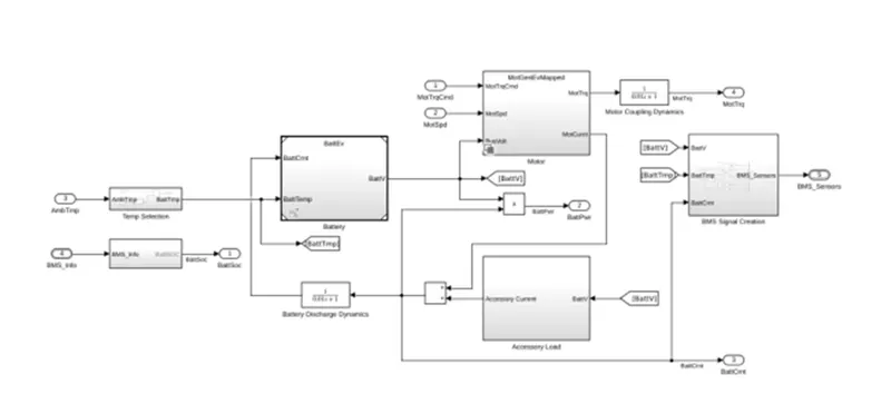
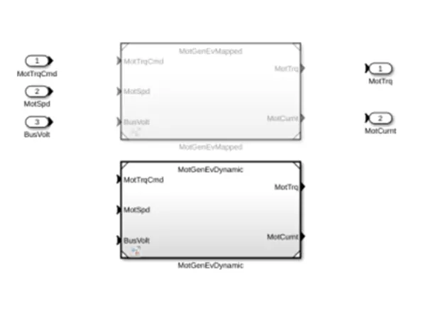
• Then select the ‘MovGenEV mapped’ block.

• From the below figure it is clear that by default mapped motor is selected.

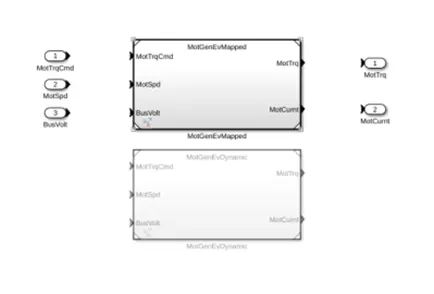
• Now, changing the mapped to dynamic blockset, right click on the screen and select variant. The label the mode active choice and select MotGenEvdynamic.

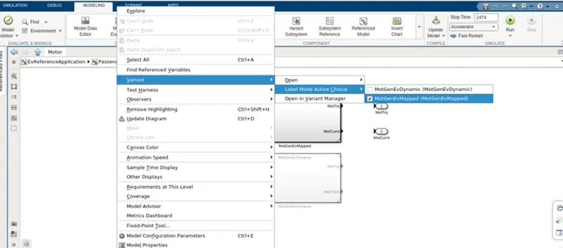
• Similarly, we can change from dynamic to mapped by selecting MotGenmapped option.

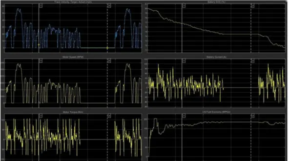
RESULTS: By clicking on the run the results obtained when FTP75 drivecycle is used with similar line of 2474 seconds.

Q2. How does the model calculate miles per gallon? Which factors are considered to model fuel flow?

MILES PER GALLON:

MPG is a fuel economy rating determined by how far a car can travel on a gallon of gasoline or diesel. Although the metric version would be kilometres per litre, MPG is adopted In many system countries like Canada.

While it is both cheaper and better for the environment to achieve a higher MPG rating, there is a curve, that the EPA calls the “MPG illusions” that shows the cost benefits of increasing MPG decrease with higher rating.

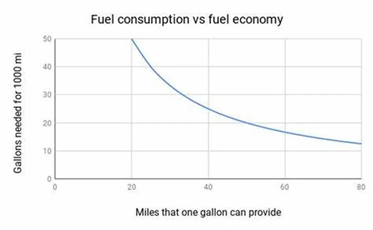
Because, of this “car illusion”, car makers in both United states and Canada are beginning to list their cars mileage in fuel consumption per distance. In Canada, this is done in litres per 100 kilometres (L/100Km), and in the USA, this is done in gallons per 100 miles (gal/100mi).

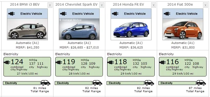
From above we can say that fuel economy (MPG) is high in Electric vehicles.

Calculation of miles per gallons in ‘EV Reference Application’ model:

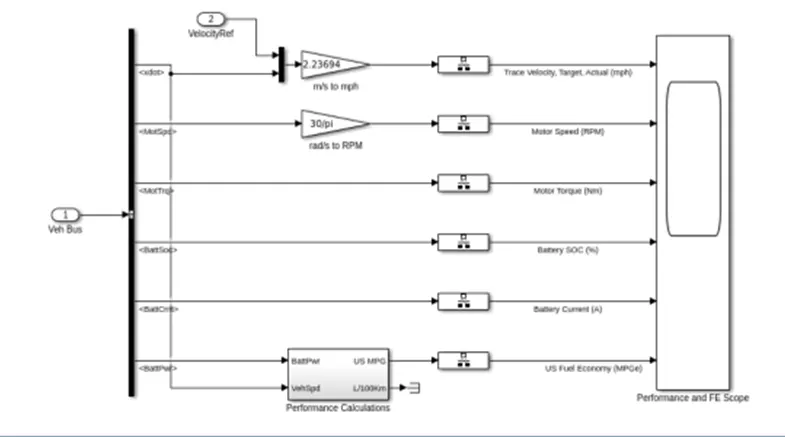
• Open the EVReference application model in the MATLAB and inside the visualisation block we can see the blocks used for calculation of MPG.
• Now open the performance calculation block.

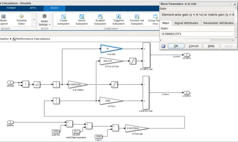
Note:

• 172US Gallons = 1000L
• 1Gallon = 33.7 Kilowatt hours of energy in electric vehicles.

• Here vehicle speed (x) is multiplied it self and the square rooted. The value is integrated (1/s) and converted into metres (m). then the metres (m) are converted into miles in the block (m to mile) then it is divided by US Gal to get US MPG.
• For US Gallon we need to divide battery power divided by 1000 and then divide by 33.7. Now, it is converted from seconds to hours by dividing with 3000 then it is converted to m^3 per Gal.
• The value is finally converted into Gallon and used as MPG after dividing miles with Gallon.

Factors considered in model fuel flow:

• Battery power capacity should be high and vehicle power consumption should be low for higher MPGe miles per Gallon is equivalent.
• Vehicle speed

Q3. Run the HEV Reference Application with WOT drive cycle. Change the grade and wind velocity in the environment block. Comment on the results

HEV Reference application with WOT drive cycles:

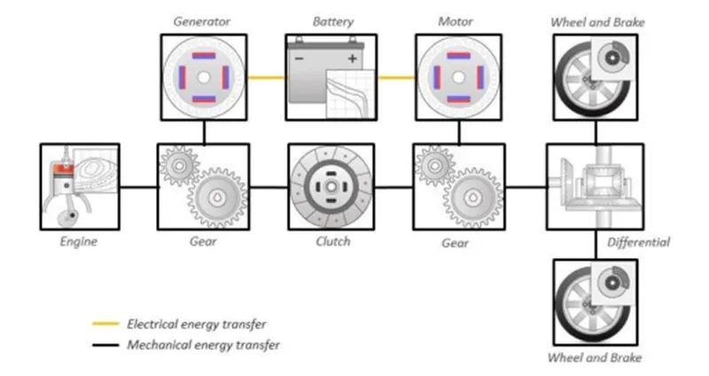
The hybrid electric vehicle reference application represents a full multimode Hybrid electric Vehicle (HEV) model with an internal combustion engine, transmission, battery, motor, generator, and associated powertrain control algorithms. Use the reference application for powertrain matching analysis and component selection, control and diagnostic algorithms design, and hardware- in- loop (HIL) testing.

By default, the HEV multimode reference application is configured with,

• Mapped motor and generator
• 5L_spark_ignation (SI) dynamic engine

The diagram shows the powertrain configuration

HEV Reference application model:

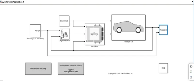
Description:

• Open ‘HEV Reference application’ model in MATALB
• It consists of various subsystems which are similar to ‘EV Reference application’ but the complexity is more than in ‘HEV Reference application’ model.

Case 1:

The default drive cycle is FTP75 with 2474 sec. Now change into WOT drive cycle as below with WOT simulation time as 180 sec and click on OK.

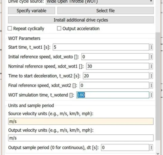
Result:

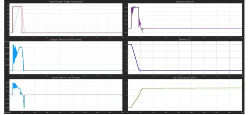
• The target velocity actual was able to achieve 67.1 mph. the battery current was increased up to 500 Amp and maintained for a duration of 14 sec.
• Engine speed is able to achieve 8000 RPM and battery state of charge (soc) was decrease from 80 to 72.
• Engine torque increases initially and goes to negative after 20^th second and the peak torque achieve was around 275 Nm. Fuel economy was increased initially and goes to negative after the 20^th second and the peak torque achieve was around 275 Nm. The fuel economy was increased from 0 to 16 and remains constant.

Graph1:

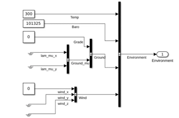
Case2:

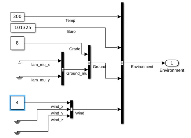
Now change the environment subsystem in case 1 specification of HEV Reference application. The grade was now changed from 0 to 8 and wind velocity from 0 to 4.

Graph2:

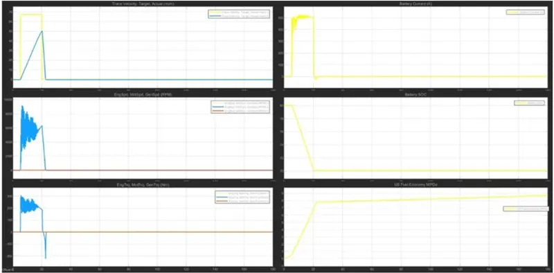
Result:

• The target velocity is actual was only able to achieve 50.4 mph. the battery current was increased up to 500 Amp and maintained for a duration of 14 sec
• Engine speed was able to achieve 8000 RPM but for a small duration of time and battery state of charge (SOC) was decrease from 80 to 70.
• Engine torque increase initially and goes to negative after 20^th second and the peak torque achieve was around 275Nm. The fuel economy was increased from 0 to 8.7 and remains constant

Q4. Keeping all other parameters same, compare the simulated results of hybrid and pure electric powertrains.

Case1: HEV multimode reference application:

• open a HEV Reference application model in MATLAB
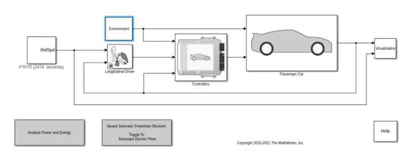
• the model consists of environment, drive cycles, longitudinal Driver passenger and Visualisation subsystems.
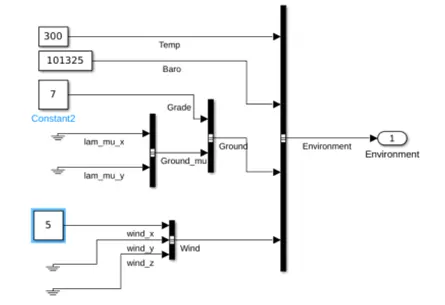
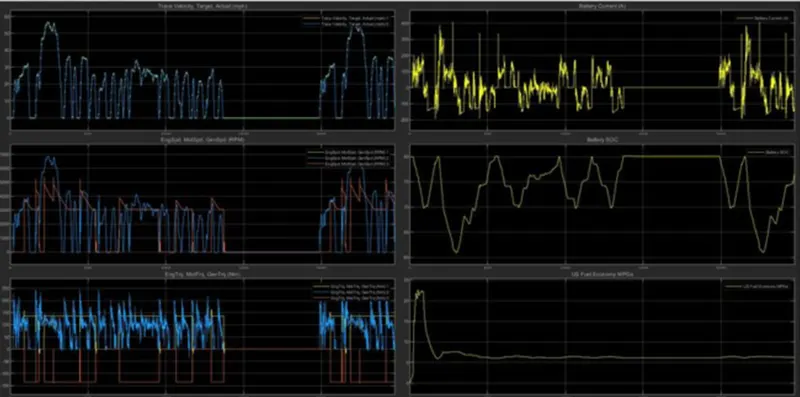
• Open the environment block and change the grade value to 7 and the velocity to 5.
• Now run the simulation with 2474 seconds and go to the visualisation to see the graph.

Model:

Result graph:

Case 2: EV Reference application model

• Open Electric vehicle Reference application model in MATLAB
• The model consists of environment, drive cycles, longitudinal Driver passenger and Visualisation subsystems similar to the HEV but as it is a pure electric vehicle the complexity in the model is less and the rendering time is less.
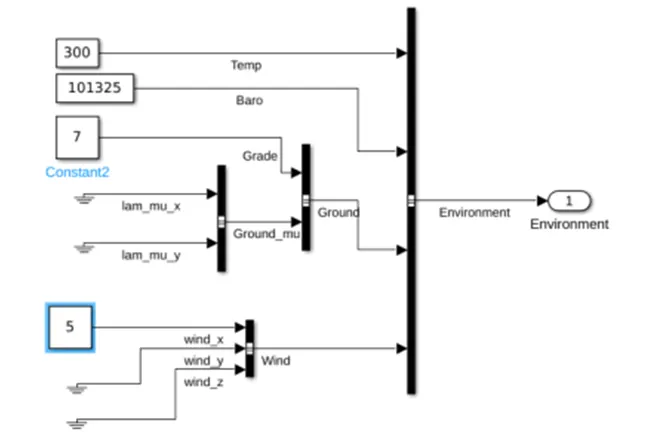
• Open the environment block and change the grade value to 7 and the velocity to 5.
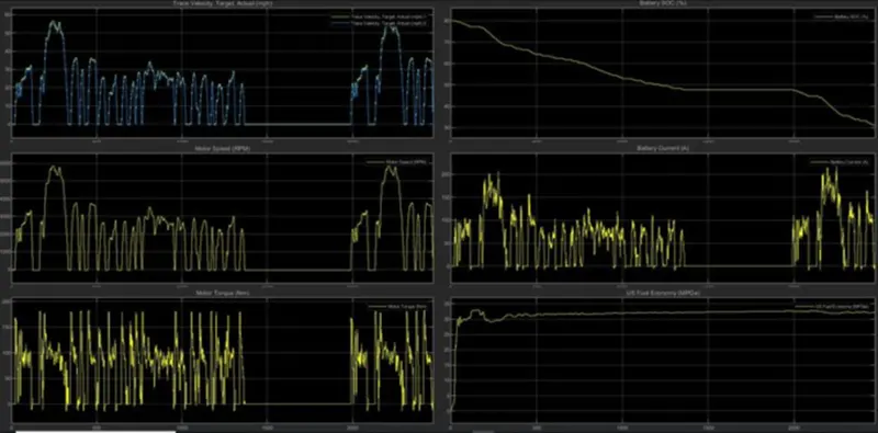
• Now run the simulation with 2474 seconds and go to the visualisation to see the graph.

Model:

Result Graph:

Conclusion:

• The battery current is continuously changing in HEV due to charging and discharging while in pure EV the battery current is continuously dropping.
• The motor speed (RPM) is high for HEV compared to EV.
• The US fuel economy is high in EV compared to HEV, travelling cost is less for EV.