Week-4 Challenge WOT Condition Part-2
AIM: To do the simulation on HevReferenceApplication and EvReferenceApplication Simulink layout and observe the results.
OBJECTIVE:
- Note the differentiated between the mapped and dynamic model of engine, motor and generator and showed how to change the required model type setting.
- Explain how the unit calculation is done to miles per gallon and factors considered to model the fuel flow.
- Run the simulation on HevReferenceApplication layout by choosing the WOT drive cycle and changing the environmental values of grade and wind speed in x-direction and observed the results.
- Compares the HevReferenceApplication and EvReferenceApplication and plot the results.
THEORY:
Powertrain block set will provide fully assembled reference application models of automotive powertrains, which includes gasoline, diesel, hybrid and electric systems. It includes a component library for simulating engine subsystems, transmission assemblies, traction motors, battery packs and controller models. It also includes a dynamometer model for virtual testing.
We can use this block set for design trade-off analysis and component sizing, control parameter optimization and hardware-in-the-loop testing.
1. What is the difference between mapped and dynamic model of engine, motor and generator? How can you change model type?
|
Mapped model (Engine, Motor and Generator) |
Dynamic model (Engine, Motor and Generator) |
|
Model uses a set of steady-state lookup tables to characterize engine, motor and generator performance. |
The model uses actual component data to characterize the engine, motor and generator performance. |
|
The tables provide overall engine, motor and generator characteristics. |
They are suitable to run the diagnostics or controlling the design parameters and are suitable for running. |
|
Mapped models are faster while running the simulation. |
Dynamic models are slower while running the simulation. |
Changing Model Path
In the EvReferenceApplication Simulink layout, by default mapped motor model is selected.
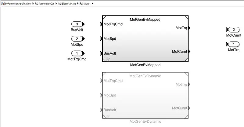
In order to change the model, follow the below steps
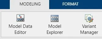
- In the Simulink layout interface, go to the modelling browser and select the Variant Manager.
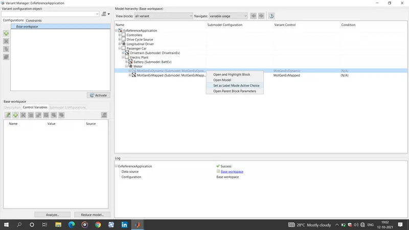
- Now, new Variant Manager interface will open and in the Electric plant open the motor system and right click on the sub-model (Mapped motor or generator) then choose the Set as Label Mode Active Choice, the changes will be applied in the model.
2. How does the model calculate miles per gallon? Which factors are considered to model fuel flow?
In the EvReferenceApplication Simulink layout open the Visualization block in that again open the Performance Calculations sub-block and observe the unit’s conversions.
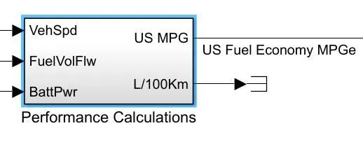
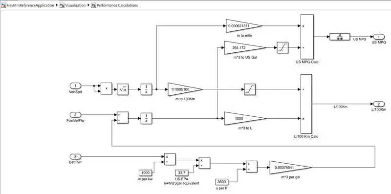
- Vehicle speed, Fuel volume flow and Battery power are the 3 important values for this unit conversion.
- Vehicle speed is converted to miles and divided by US gal to bring out miles per gallon (MPG) value.
- Where Battery power in watts converted to KW by dividing with 1000 and resulted value is again converted to US EPA kw/USgal equivalent by dividing with 33.7 and again the resulted value is converted to hour by dividing with 3600. So, we got m^3 per gal value with multiplication of gain 0.00378541.
- We can add this value with direct fuel used by the engine and integrate sum to volume in m^3.
- Now the resulted value is multiplied with 264.172 to convert from m^3 to US Gal.
- Finally, the vehicle speed in miles is divided with US Gal value to bring out miles per gallon (MPG) value.
Factor considered to model fuel flow
- Vehicle speed
- Fuel Volume Flow
- Battery Power
3. Run the HEV Reference Application with WOT drive cycle. Change the grade and wind velocity in the environment block. Comment on the results.
HEV Reference Application with WOT drive cycle
The default drive cycle is FTP75, now we need to change the drive cycle.
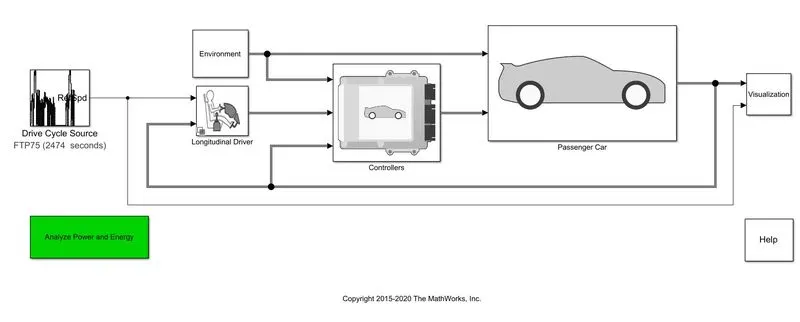
For the Wide-Open Throttle (WOT) drive cycle
- Normal vehicle speed is 40 mph
- Time for starting deceleration is 45 seconds
- Simulation time 120 seconds
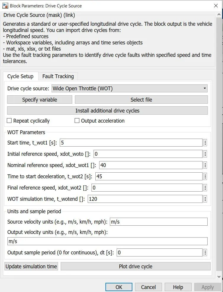
Layout
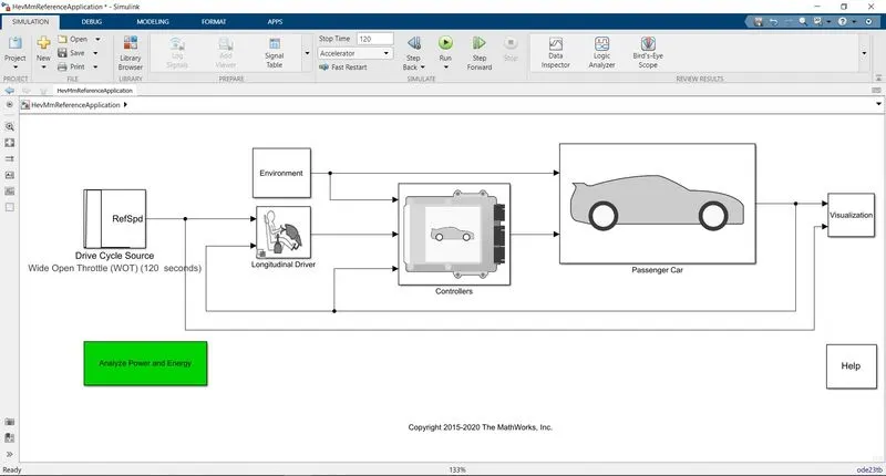
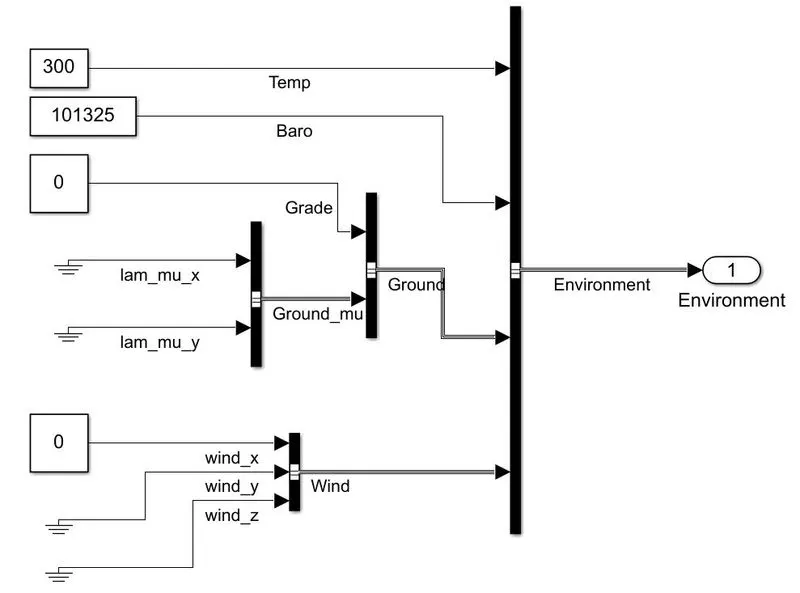
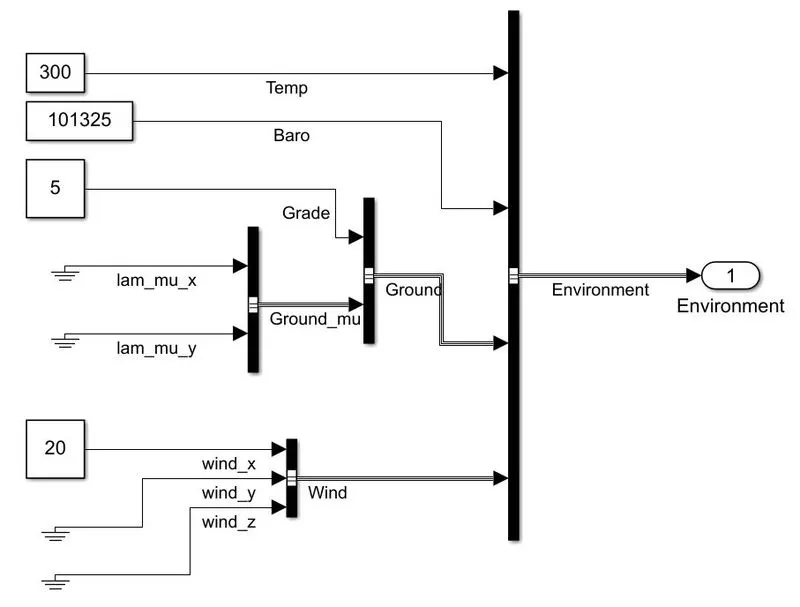
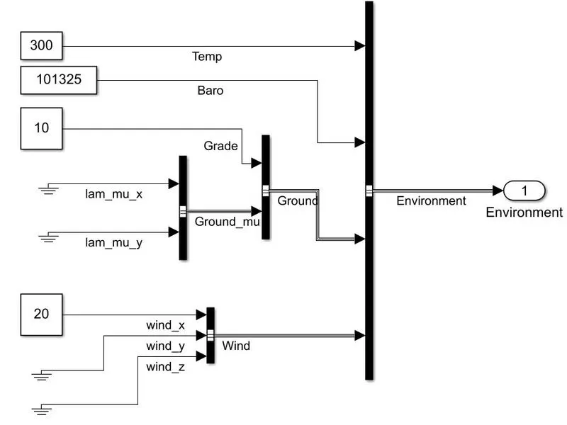
So, for better understanding of the simulation results we have changed the gradeability and wind velocity values for the vehicle in the environment block.
Condition-1: Gradeability-0 and Wind Velocity-0
Results:
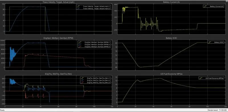
Plot-1: Initially the vehicle speed will be 0 mph from 0-5 seconds, after 5 seconds speed increases gradually and reaches a maximum speed of around 85 mph in 22 seconds and remains constant still the deceleration starts, when the deceleration starts the vehicle speed decreases gradually and remains constant.
Plot-2: we can notice that plot is related to engine (yellow), motor (blue) and generator (red) speeds. Motor gets the energy from the battery source and the motor speed increases still the vehicle attain its maximum speed and almost remains constant still the deceleration time. The engine and generator speed are almost constant through the simulation where they start after 22 seconds and rapidly increases, there will be gradual decrease still 88 seconds then rapidly decreases and remains constant.
Plot-3: This plot is related to torque of engine, motor and generator. Generally, we can say this plot will be opposite to speed plot. After 45 seconds the motor speed reduces suddenly so, the motor torque gets reversed (negative toque) then the battery gets charged up the SOC increases gradually. The engine torque and generator toque values are opposite to each other.
Plot-4: This plot shows battery current values we can notice that as the motor peed increases the current also increases and vice-versa during deceleration the current values will be in negative values and battery gets charged.
Plot-5: This plot shows the State of Charge (SOC) values. Initially the SOC is 80%, after 5 seconds motor speed increases then the SOC reduces gradually still the motor speed attains the constant value. After 45 seconds motor speed decreases gradually and the battery gets charged up means SOC increases gradually up to the speed on the engine, motor and generator are almost 0 rpm.
Plot-6: This plot shows the US fuel economy in miles per gallon (MPG). After 5 seconds the fuel usage by the engine will increase gradually as the vehicle speed increases, After 45 seconds the vehicle will decelerate which means the fuel usage will reduce gradually and remains constant after the engine attains 0 rpm.
Condition-2: Gradeability-5 and Wind Velocity-20
Results:
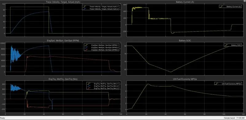
When the gradeability and wind speed in increased we can notice that vehicle will take more time to reach maximum speed. Maximum speed is around 73 mph and taken almost 37 seconds.
Condition-3: Gradeability-10 and Wind Velocity-20
Results:
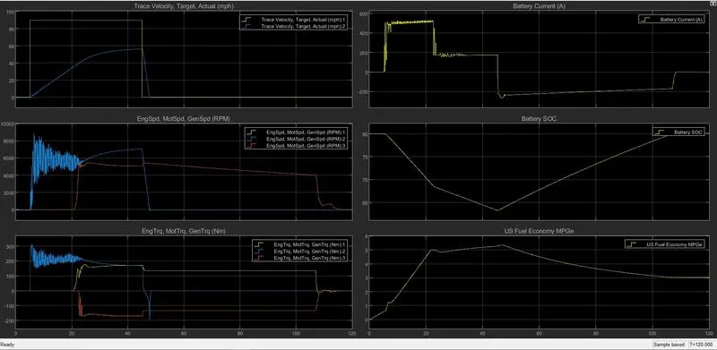
As the gradeability is increases further with constant wind speed we can notice that maximum speed of the vehicle is 56 mph and taken 38 seconds to reach this speed.
Finally, we can conclude that with increase in Gradeability and wind speed the following observations are made
- The maximum velocity (mph) achieved is reduced with respect to time.
- As the deceleration time reduces the battery charging capacity will be reduced.
- During deceleration the SOC increases because the motor and generator torque values are in negative.
- Fuel economy will reduce because the distance travelled will be less due to external force (wing speed) acting on the vehicle.
4. Keeping all other parameters same, compare the simulated results of hybrid and pure electric powertrains.
Comparing HEV and EV Powertrains systems
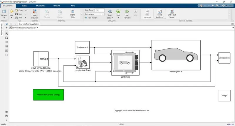
HevReferenceApplication Simulink layout
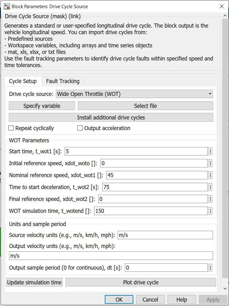
Chosen Wide Open Throttle (WOT) drive cycle for the simulation where grade and wind Speed are ‘0’
- Normal vehicle speed is 45 mph
- Time for starting deceleration is 75 seconds
- Simulation time 150 seconds
Layout
Results:
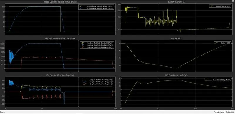
- The maximum velocity of the vehicle is around 100 mph and it takes about 32 seconds, then vehicle maintain this velocity for 75 seconds and deceleration of the vehicle starts.
- Time taken during Deceleration is 5 seconds.
- SOC of the battery decreases still the deceleration of the vehicle start. During deceleration the motor toque, generator toque and battery current values will enter to the negative zone, so SOC will increase gradually and attain the peak value.
- SOC at the start and at the end is almost same.
- Maximum US fuel economy is 13.3 MPGe
Engine plant
Electric plant
Drivetrain plant
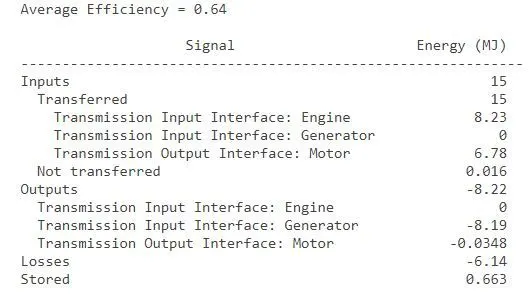
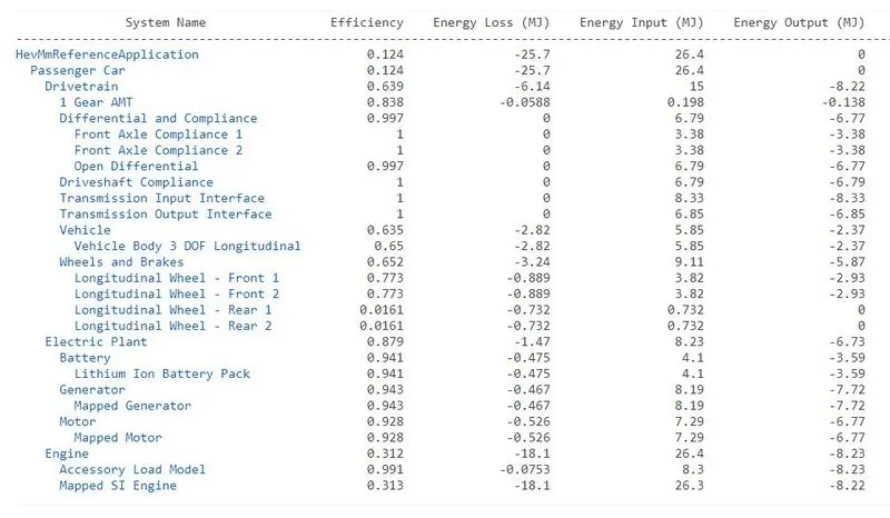
Overall plant HEV summary
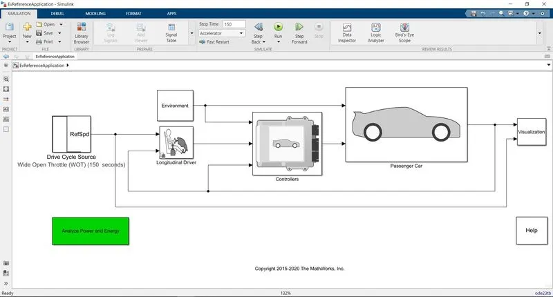
EvReferenceApplication Simulink layout
Layout
Results:
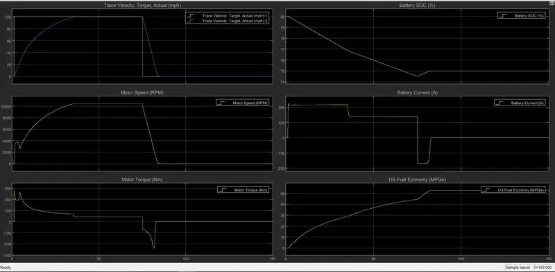
- The maximum velocity of the vehicle is around 100 mph and it takes about 37 seconds, then vehicle maintain this velocity for 75 seconds and deceleration of the vehicle starts.
- Time taken during Deceleration is 8 seconds.
- SOC of the battery decreases still the deceleration of the vehicle start. During deceleration the motor toque and battery current values will enter to the negative zone, so SOC will increase gradually and attain the peak value.
- SOC at the start (80%) and at the end (75%) is not same.
- Maximum US fuel economy is 53 MPGe
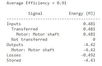
Electric plant
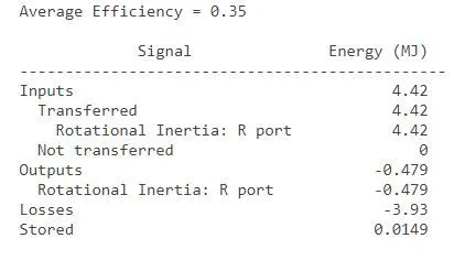
Drivetrain plant
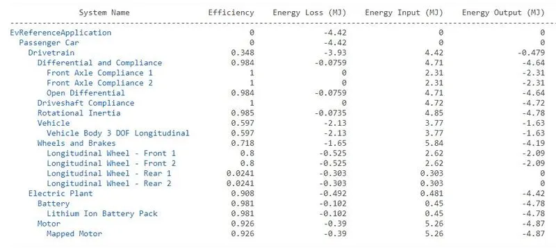
Overall plant summary
Finally, by observing the results we can say that
- HEV runs with two power sources Engine (CI/SI) and Battery whereas EV runs with only Battery power source.
- The total time taken to reach the maximum velocity is less for HEV (34 seconds) as compared to EV (37 seconds)
- The deceleration time is also less for HEV because it has many moving frictional parts compared to EV.
- US fuel economy is more for EV (53 MPGe) when compared to HEV because EV has less number of moving parts which means it has low frictional losses.
- SOC of the EV will not be same at the beginning and at the end of the drive cycle whereas for HEV it is almost same.
|
Efficiency of the Plants used in the HEV and EV |
||
|
Name of the Plant |
HEV |
EV |
|
Engine |
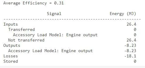
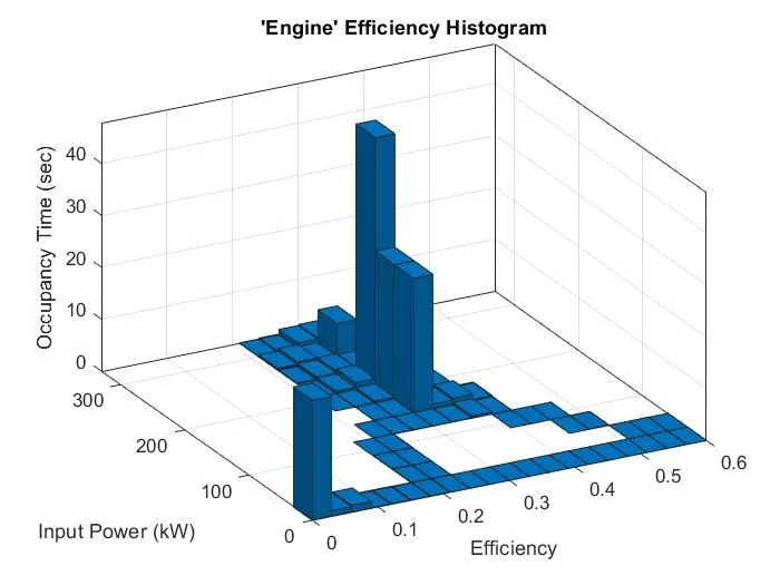
0.31 |
- |
|
Electric |
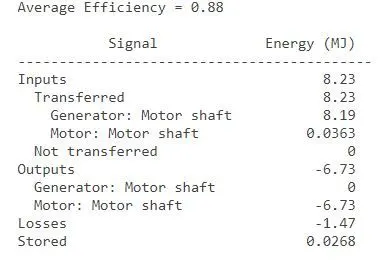
0.88 |
0.91 |
|
Drivetrain |
0.64 |
0.35 |
CONCLUSION:
Hence, we have completed the simulation on HevReferenceApplication and EvReferenceApplication Simulink layout and plotted the results as per the given condition.
- Differentiated between the mapped and dynamic model of engine, motor and generator and showed how to change the required model type setting.
- Explained how the unit calculation is done to miles per gallon and factors considered to model the fuel flow.
- We have run the simulation on HevReferenceApplication layout by choosing the WOT drive cycle and changing the environmental values of grade and wind speed in x-direction and observed the results.
- Finally, we have compares the HevReferenceApplication and EvReferenceApplication and plotted the results with detailed explanation.
REFERENCES: