Project 2 - Rankine cycle Simulator
AIM
To write a program for Simulation of Rankine cycle
OBJECTIVES
- Program Code should calculate the state points of the Rankine Cycle.
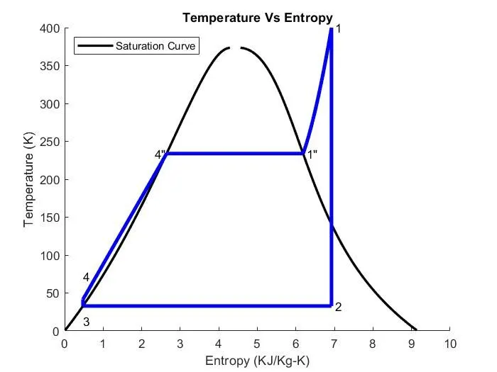
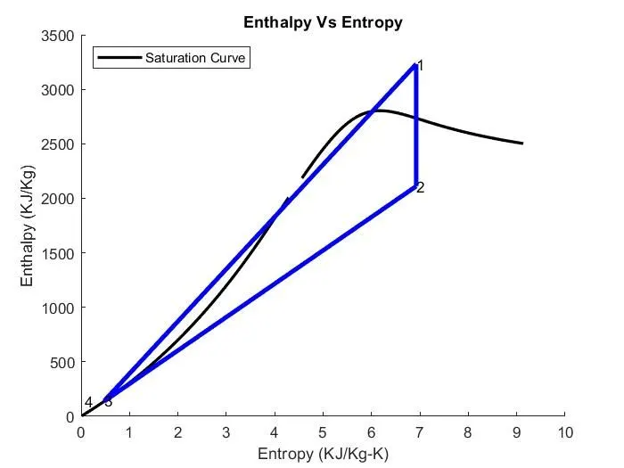
- Plot the corresponding T-s and h-s plots for the given set of inputs.
THEORY
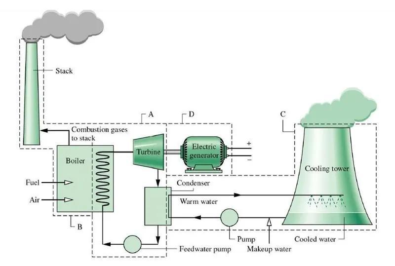
Rankine cycle is an idealized thermodynamic cycle describes the process by certain heat engines, such as steam turbines or reciprocating steam engines, which allows mechanical work to be extracted from a fluid as it moves between a heat source and heat sink.
Heat energy (coal) is supplied to the boiler, with the help of coal handling system. The working fluid (water) is pumped to the boiler tubes and converted to a high pressure gaseous state (steam). In order to run the turbine, the high pressurized steam is expanded in the turbine. After passing over the turbine the fluid is allowed to condense back into a liquid state as waste heat energy is rejected before being returned to boiler, this completes the cycle.
In larger systems, the frictional losses are neglected for the purpose of simplifying the calculations and these losses are usually have less significant then thermodynamic losses.
Thermal power plant layout
T-S diagram
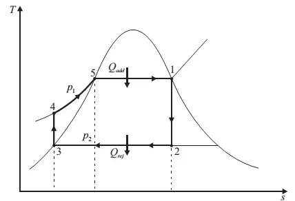
4-Processes in Rankine Cycle
1-2 is Isentropic Expansion in Turbine
High pressurized vapour from the boiler output enters the turbine at state-1, where the vapour expands isentropically over the turbine fixed and moving blades to develop work by the mechanical rotation of the turbine shaft, which is further connected to the electrical generator.
- Workdone by the turbine
W_turbine = h1-h2 KJ/Kg
2-3 is Constant pressure heat rejection in Condenser
Vapour enters the condenser at state-2.In the condenser the phase chage occurs as vapour is condensed to liquid at constant pressure, by transfering the steam's heat to the circulating water flow through the tubes of the condenser. Phase change occurs in the condenser, and the working fluid leaving the condenser is in a liquid state.
- Heat rejected in the condenser
Q_out = h2-h3 KJ/Kg
3-4 is Isentropic Compression in Pump
Working liquid exits the condenser at state-3 and enters in to the pump. Pump increases the pressure of the working liquid by imparting work during the process. In some plant units of smaller size and low specific volumes, this small work can be neglected compared to the work output os a steam turbine.
- Workdone by the pump
W_pump = h4-h3 KJ/Kg
4-1 is Constant pressure heat Addition in Boiler
Boiler is an large heat exchanger where heat is liberated by the combursion of fuels like coal, oil and lignite will transfer the haet indirectly to the working fluid at constant pressure. Here water enters the steam boiler from the boiler feed pump as a compressed liquid at state-4 and is heated to the saturation temperature i.e state-1.
- Heat supplied to Bioler
Q_in = h1-h4 KJ/Kg
Formulas
W_net = W_turbine - W_pump KJ/Kg
Thermal Efficiency = (W_net / Q_in)*100 %
Specific fuel consumption = 3600 / W_net KJ/KW-hr
Work ratio = W_net / W_turbine
Back work ratio = W_pump / W_turbine
How to Increase Thermal efficienty of the power plant
- By increasing the Boiler pressure
- Superheating the steam to high temperature
- Lowering the Condenser pressure
Main Program for the Simulation of Rankine Cycle
% Writing a Program to Simulate Rankine Cycle
clear all
close all
clc

% Displaying the processes involved in the Rankine cycle
disp('           RANKINE CYCLE SIMULATION           ')
disp('1-2 is Isentropic Expansion in the Turbine')
disp('2-3 is Constant pressure Heat Rejection by the Condenser')
disp('3-4 is Isentropic Compression in the Pump')
disp('4-1 is Constant pressure Heat Addition by the Boiler')

% Entering the input values in the command window
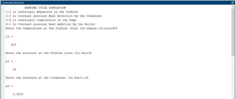
t1 = input('Enter the Temperature at the Turbine inlet (in Degree Celsius)')
p1 = input('Enter the Pressure at the Turbine inlet (in bar)')
p2 = input('Enter the Pressure at the Condenser (in bar)')

% Calling the 'Xsteam' function for the valued of Enthalpy and Entropy at liquid and vapour states
%State-1 (Boiler outlet to Turbine inlet)
h1 = XSteam('h_pT',p1,t1);      %h_pT	Entalpy as a function of pressure and temperature.
s1 = XSteam('s_pT',p1,t1);      %s_pT	Specific entropy as a function of pressure and temperature (Returns saturated vapour entalpy if mixture.)

% State-2 (Turbine outlet to Condenser input)
s2 = s1;
t2 = XSteam('Tsat_p',p2);       %Tsat_p	Saturation temperature
hf2 = XSteam('hL_p',p2);        %hL_p	Saturated liquid enthalpy
hg2 = XSteam('hV_p',p2);        %hV_p	Saturated vapour enthalpy
sf2 = XSteam('sL_p',p2);        %sL_p	Saturated liquid entropy
sg2 = XSteam('sV_p',p2);        %sV_p	Saturated vapour entropy
x2 = ((s2-sf2)/(sg2-sf2));
h2 = hf2+(x2*(hg2-hf2));

% State-3 (Condenser output to Pump input)
p3 = p2;
t3 = XSteam('Tsat_p',p3);       %Tsat_p	Saturation temperature
h3 = XSteam('hL_p',p3);         %hL_p	Saturated liquid enthalpy
s3 = XSteam('sL_p',p3);         %sL_p	Saturated liquid entropy

% State-4 (pump outlet to Boiler inlet)
p4 = p1;
s4 = s3;

% Defining gamma at state-4
% gamma_4 = Cp_4/Cv_4
Cp_4 = XSteam('Cp_ps',p4,s4);   %Cp_ps	Specific isobaric heat capacity as a function of pressure and entropy.
Cv_4 = XSteam('Cv_ps',p4,s4);   %Cv_ps	Specific isochoric heat capacity as a function of pressure and entropy.
gamma_4 = (Cp_4/Cv_4);
g = (gamma_4 -1/gamma_4);

t4 = t3*((p4/p3)^g);
h4 = XSteam('h_ps',p4,s4);      %h_ps	Entalpy as a function of pressure and entropy.

% Workdone in the Turbile(Wt)
Wt = h1-h2;

% Workdone in the pump(Wp)
Wp = h4-h3;

% Net Workdone per one cycle
W_net = Wt-Wp;

% Heat supplied to the boiler
Q_in = h1-h4;

% Heat rejected by the boiler
Q_out = h2-h3;

% Thermal efficiency of the power plant
Thermal_Efficiency = (W_net/Q_in)*100;

% Specific fuel consumption (SFC)
SFC = 3600/W_net;

% Work ratio
Work_ratio = W_net/Wt;

% Back work ratio
Back_work_ratio = Wp/Wt;

% values of t,h and s at saturated liquid and vapour lines
tf = XSteam('Tsat_p',p1);       %Tsat_p	Saturation temperature
hf = XSteam('hL_p',p1);         %hL_p	Saturated liquid enthalpy
sf = XSteam('sL_p',p1);         %sL_p	Saturated liquid entropy
hg = XSteam('hV_p',p1);         %hV_p	Saturated vapour enthalpy
sg = XSteam('sV_p',p1);         %sV_p	Saturated vapour entropy

% Plotting Temperature-Entropy (T-S) diagram
figure(1)
hold on
T = linspace(0,400,500);
for i = 1:length(T)
    SL(i) = XSteam('sL_T',T(i));    %sL_T	Saturated liquid entropy
end

for j= 1:length(T)
    SV(j) = XSteam('sV_T',T(j));    %sV_T	Saturated vapour entropy
end

plot(SL,T,'linewidth',2,'color','k');
plot(SV,T,'linewidth',2,'color','k');

T = XSteam('Tsat_p',p1);        %Tsat_p	Saturation temperature
t = linspace(T,t1,500);

for i = 1:length(t)
    S(i) = XSteam('s_pT',p1,t(i));  %s_pT	Specific entropy as a function of pressure and temperature (Returns saturated vapour entalpy if mixture.)
end

t5 = XSteam('Tsat_p',p4);       %Tsat_p	Saturation temperature
s5 = XSteam('sL_T',t5);         %sL_T	Saturated liquid entropy

plot([s1 s2],[t1 t2],'linewidth',3,'color','b');
plot([s2 s3],[t2 t3],'linewidth',3,'color','b');
plot([s3 s4],[t3 t4],'linewidth',3,'color','b');
plot([s4 s5],[t4 t5],'linewidth',3,'color','b');
plot([sf sg],[tf tf],'linewidth',3,'color','b');
plot(S,t,'linewidth',3,'color','b');

xlabel('Entropy (KJ/Kg-K)');
ylabel('Temperature (K)');
title('Temperature Vs Entropy');
legend('Saturation Curve','location','northwest');

% Indicating the state points
text(s1+0.1,t1,'1');
text(s2+0.1,t2,'2');
text(s3,t3-20,'3');
text(s4,t4+30,'4');
text(s5-0.3,t5,'4"');
text(sg+0.1,tf,'1"');

% Plotting Enthalpy-Entropy (H-S) diagram
figure(2)
hold on

T1 = linspace(0,400,500);
for i = 1:length(T1)
    HL(i) = XSteam('hL_T',T1(i));       %hL_T	Saturated liquid enthalpy
end
for j= 1:length(T1)
    HV(j) = XSteam('hV_T',T1(j));       %hV_T	Saturated vapour enthalpy
end

plot(SL,HL,'linewidth',2,'color','k');
plot(SV,HV,'linewidth',2,'color','k');

plot([s1 s2],[h1 h2],'linewidth',3,'color','b');
plot([s2 s3],[h2 h3],'linewidth',3,'color','b');
plot([s3 s4],[h3 h4],'linewidth',3,'color','b');
plot([s4 s1],[h4 h1],'linewidth',3,'color','b');
xlabel('Entropy (KJ/Kg-K)');
ylabel('Enthalpy (KJ/Kg)');
title('Enthalpy Vs Entropy');
legend('Saturation Curve','location','northwest');

% Indicating the state points
text(s1,h1+1,'1');
text(s2,h2+1,'2');
text(s3-0.2,h3,'3');
text(s4+0.3,h4,'4');

% Printing the output for 4 state's
disp('RESULTS')

%Printing State point-1
disp('At State Point 1:')
fprintf('P1 is : %f bar\r\n',p1)
fprintf('T1 is : %f Degree Celsius\r\n',t1)
fprintf('H1 is : %f KJ/Kg\r\n',h1)
fprintf('S1 is : %f KJ/Kg-K\r\n',s1)

%Printing State point-2
disp('At State Point 2:')
fprintf('P2 is : %f bar\r\n',p2)
fprintf('T2 is : %f Degree Celsius\r\n',t2)
fprintf('H2 is : %f KJ/Kg\r\n',h2)
fprintf('S2 is : %f KJ/Kg-K\r\n',s2)
fprintf('X2 is : %f \r\n',x2)

%Printing State point-3
disp('At State Point 3:')
fprintf('P3 is : %f bar\r\n',p3)
fprintf('T3 is : %f Degree Celsius\r\n',t3)
fprintf('H3 is : %f KJ/Kg\r\n',h3)
fprintf('S3 is : %f KJ/Kg-K\r\n',s3)

%Printing State point-4
disp('At State Point 4:')
fprintf('P4 is : %f bar\r\n',p4)
fprintf('T4 is : %f Degree Celsius\r\n',t4)
fprintf('H4 is : %f KJ/Kg\r\n',h4)
fprintf('S4 is : %f KJ/Kg-K\r\n',s4)

% Formulas output
fprintf('Workdone by the Turbine : %f KJ/Kg\r\n',Wt)
fprintf('Workdone by the Pump : %f KJ/Kg\r\n',Wp)
fprintf('Heat added in to the Boiler : %f KJ/Kg\r\n',Q_in)
fprintf('Heat rejected in Condenser : %f KJ/Kg\r\n',Q_out)
fprintf('Thermal Efficiency of the Power Plant : %f %%\r\n',Thermal_Efficiency)
fprintf('Specific fuel consumption : %f KJ/KW-hr\r\n',SFC)
fprintf('Work ratio : %f \r\n',Work_ratio)
fprintf('Back Work ratio : %f \r\n',Back_work_ratio)
Explanation
- XSteam data file contains water and Steam properties from (0 - 1000) bar and (0 - 2000) deg C of Enthalpy and Entropy at particular pressure and temperature for saturated liquid and vapour conditions.
- Displaying the 4 processes involved in Rankine Cycle.
- Next entering the input parameter in the command window
t1 = Enter the Temperature at the Turbine inlet (in Degree Celsius)
p1 = Enter the Pressure at the Turbine inlet (in bar)
p2 = Enter the Pressure at the Condenser (in bar)
- Now we have to call the 'XSteam' function to find out the state points of the Rankine cycle.
example:
h1 = XSteam('h_pT',p1,t1);
where 'h_pT' is an 'Entalpy as a function of pressure and temperature'.
In this way remaining functions were called according to the state points - which contains properties like Temperature (t), Enthalpy (h), Entropy (s) and dryness fraction (x).
- Then given the formulas (Standard Thermodynamic relations) for the calculation of Turbine and pump work, Net workdone, Heat input and output, Thermal efficiency, Specific fuel consumption, Work ratio and Back work ratio.
- Extracted the values of t, h and s at saturation liquid and vapour line for plotting i.e from state 4-4''.
- By defining the temperature range (T) and using 'for loop' Saturation curve for liquid and vapour are plotted.
- Plotted T-S diagram from the defined data with proper label's, title and legends.
- Indicated the state points with 'numbers', using 'text' command and adjusted the position of the number.
example:
text(s1+0.1,t1,'1');
where s and t are the state points and indicated with number '1'
'+0.1' means adjusting the number '1' (It moves upward) for proper apperance. Even '-' sign can be used to move the number '1' downward.
- Then Plotted H-S diagram from the defined data with proper label's, title and legends.
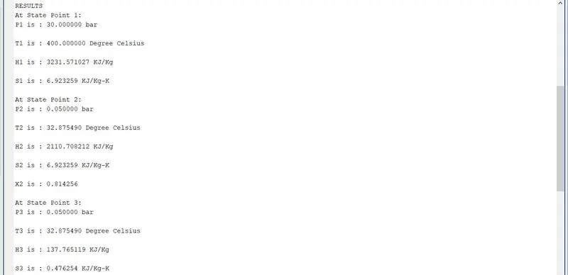
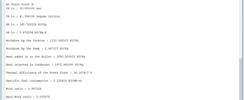
- Finally, printed all the state point (4) properties (Temperature (t), Enthalpy (h), Entropy (s) and dryness fraction (x)) and Turbine and pump work, Net workdone, Heat input and output, Thermal efficiency, Specific fuel consumption, Work ratio and Back work ratio.
- These values will be displayed in the command window after entering the input values of t1, p1 and p2.
OUTPUT
T-S Diagram
H-S Diagram
Command Window inputs and Results
Errors
- Only typing error have been encountured.
- After running the program those errors have been corrected.
References