Week-4 Challenge WOT Condition Part-2

Objective:

1. What is the difference between the mapped and dynamic model of engine, motor and generator? How can you change the model type?

2. How does the model calculate miles per gallon? Which factors are considered to model fuel flow?

3. Run the HEV ReferenceApplication with WOT drive cycle. Change the grade and wind velocity in the environment block. Comment on the results.

4. Keeping all other parameters same, compare the simulated results of hybrid and pure electric powertrains.

Solution of objective-1:

Difference between Mapped and Dynamic System-

S. No.	Mapped	Dynamic
1	Mapped engines represent macro engine behaviour as a set of lookup tables (brake torque, fuel flow, air mass flow, exhaust temperature, efficiency, and emissions) as functions of commanded load and measured engine speed.	Dynamic engines decompose engine behaviour into individual component models that account for engine dynamics, most notably intake airflow and turbocharger dynamics.
2	Mapped engine models are suitable for analysis and design activities that do not require engine subsystem dynamic characteristics. For example: in engine and transmission powertrain matching analysis for fuel economy, emissions, and performance trade-offs.	Dynamic engine models are suitable for designing control, estimator, and diagnostic algorithms that depend on dynamic subsystem states. For example: in closed-loop AFR control algorithm development.
3	For quasi steady-state engine simulations.	To analyse the impact of individual engine components on the overall performance.
4	If you have engine data from a dynamometer or a design tool like GT-POWER.	If you need a more detailed dynamic model and have component-level data.

How can you change the model type?

Steps:

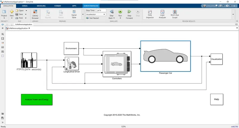
1. Run Simulink and then click on ‘Examples’ and search ‘Powertrain Blockset’ and open the ‘EV Reference Application’ example. Wait for few seconds to load the example. The example will look like this:

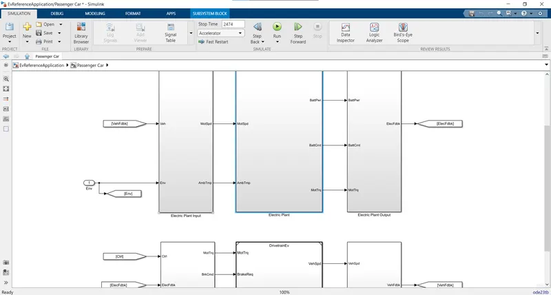
2. Double Click on Passengers block. There you will find another block named ‘Electric plant’. Open that block by double-clicking on it. In an electric plant, the block contains calculation of the battery, motor and some other blocks.

3. Open the motor block. It contains both Mapped and Dynamic block systems.

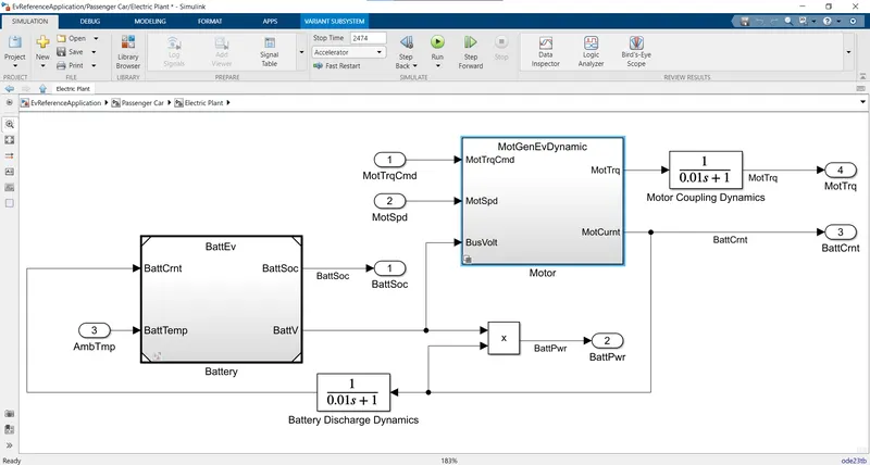
4. By default, Mapped block system is selected. To change it into Dynamic block system you have to right-click on anywhere on the screen. On right-click, you will find ‘Variant’ and click on it then click on ‘Label Mode Active Choice’ then click on ‘MotGenEvMapped’.

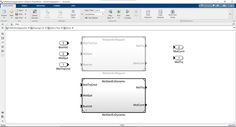
5. After that, your Mapped model will change into Dynamic model.

Solution of objective-2:

To see the model power calculations and fuel consumption calculations, go to the 'Visualization' block. In there you can find the 'Power Calculations' block. The power calculations block calculates the vehicle power or fuel consumption and its related conversions.

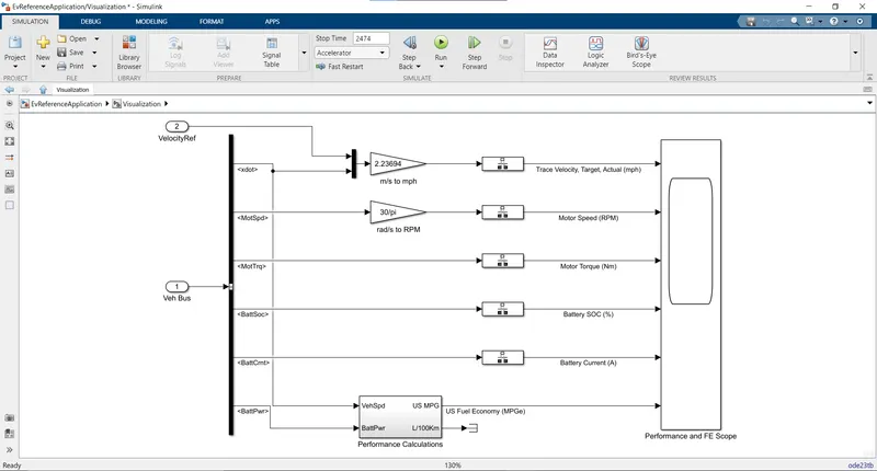
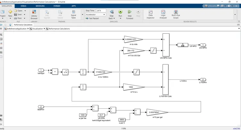
Steps to model calculate miles per gallon:

1. First, the BattPwr from port-2 is taken and divided by 1000 to convert it from watt into kilowatt and then kilowatt is divided by 33.7 to convert in kwh/USgal equivalent.

2. Then kwh/USgal equivalent is divided by 3600 to convert the second to hour.

3. After that, the value is multiplied by 0.00378541 to convert in m³/gallon and then after the integration it is multiplied by 264.172 to convert in m³ to USgal.

4. The vehicle speed is taken from the port-1 (VehSpd) and then integrate it to get the distance, and then multiplied by 0.000621371 to convert meter into mile.

5. Now the mile is divided by USgal to get the miles per gallon.

The conversions and calculations can be seen in the picture above.

Factors are considered to model fuel flow:

1. Type of vehicle

2. Type of fuel

3. Physicochemical properties of fuel

4. Fuel consumption

5. Fuel efficiency

Solution of objective-3:

HEV Reference Application with WOT cycle-

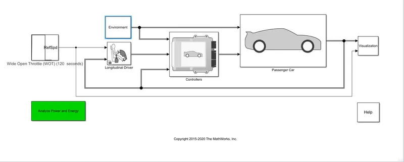
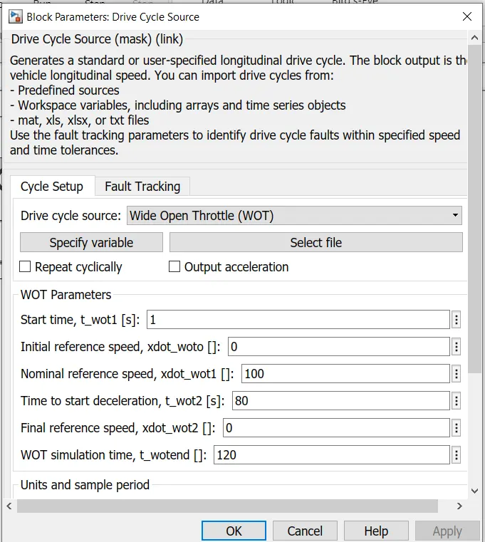
Drive Cycle Inputs-

1. Drive cycle= WOT Cycle

2. Start time = 1s and WOT simulation time=120s

3. Intitial reference speed= 0 and final reference speed= 0

4. Nominal reference speed= 100 m/s

5. Time to start deacceleration= 80 s

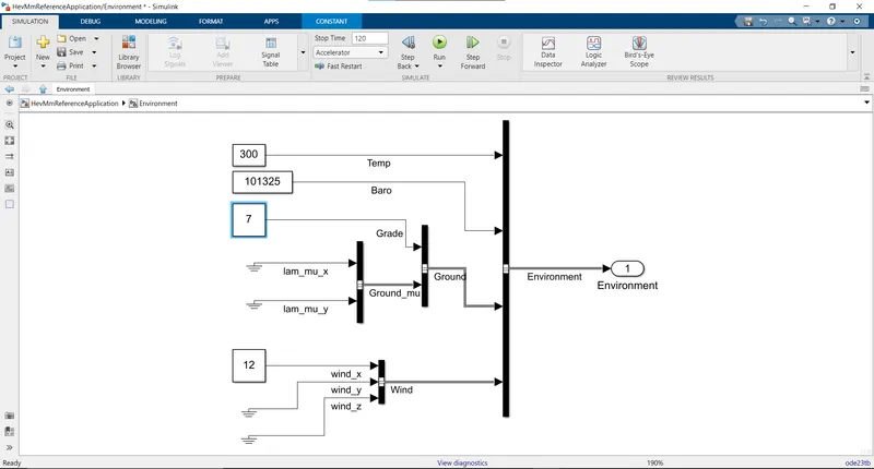
Environmental Inputs-

1. Grade=7

2. Wind velocity= 12 m/s

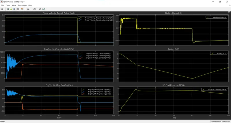
Results:

Plot-1: Trace Velocity

The targeted velocity was 100 m/s (223.694 mph) but due to the grade and wind velocity we only achieved up to 32.37m/s (72.4 mph).

Plot-2: Engine Speed, Motor Speed, Generator Speed

The second plot gives the value of the engine speed, motor speed, generator speed. It can be seen that during the acceleration period, rpm was very high and during the deceleration period it decreases.

Plot-3: Engine Torque, Motor Torque, Generator Torque

The third plot gives the value of the engine torque, motor torque, and generator torque. It can be seen that during the acceleration period, torque was increasing and during the deceleration period torque decreasing.

Plot-4: Battery Current

The fourth plot gives the information of the battery current variation.

Plot-5: Battery Soc

The fifth plot gives the information of battery Soc for drive cycle. It can be seen that Soc was decreasing during the acceleration and increasing during deceleration due to regenerative braking.

Plot-6: US Fuel Economy MPGe

The sixth plot gives the information of US fuel economy in miles per gallon equivalent. It can be seen that fuel consumption was increasing rapidly at starting of acceleration and after that, it increases at a slow rate. During the deceleration period, the fuel consumption was decreasing.

Solution of objective-4:

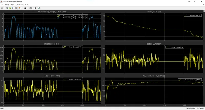
The comparison of HEV and Pure EV result is given below.

Result of HEV:

1. The target velocity is equal to the actual velocity.

2. The second plot is of engine speed, motor speed, generator speed.

3. The third plot is of engine torque, motor torque, generator torque.

4. The fourth plot is of variation in battery current.

5. The fifth plot is of battery SoC. The SoC is decreasing during acceleration and SoC is increasing during deceleration.

6. The sixth plot is of fuel consumption in USFuel Economy, MPGe.

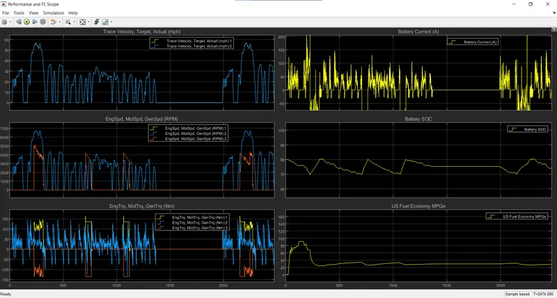
Result of Pure EV:

1. The target velocity is equal to the actual velocity.

2. The second plot is of variation in motor speed. The graphs behaviour of motor speed is the same as the trace velocity.

3. The third plot is of motor torque.

4. The fourth plot is of battery SoC. The SoC is decreasing during acceleration and SoC is increasing during deceleration.

5. The fifth plot is of variation in battery current.

6. The sixth plot is of fuel consumption in USFuel Economy, MPGe.