Project 2 - Rankine cycle Simulator

Aim: The aim of this project is to learn and understand the concept of Rankine Cycle Simulator using MATLAB.

Objective:

1. Create a Rankine Cycle Simulator using MATLAB.
2. Calculate the state points of the Rankine Cycle based on user inputs.
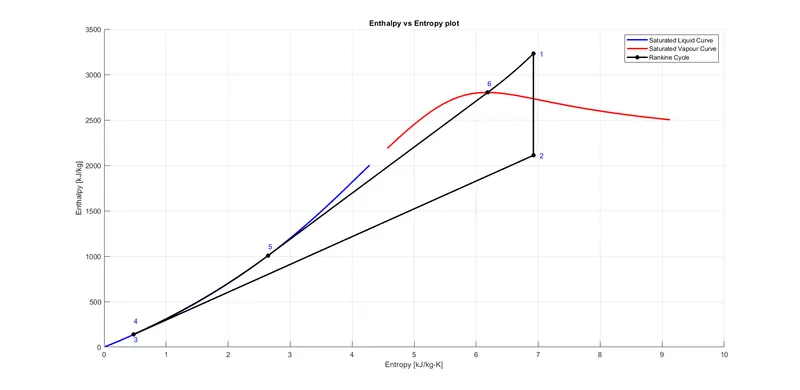
3. Plot the corresponding T-s and h-s plots for the given set of inputs. Title and axes labels are a must, while legends could be used if necessary.
4. Calculate the Net work Output and Back Work Ratio.

Theory:

Rankine Cycle:

The Rankine Cycle is a mechanical cycle commonly used in power plants to convert the pressure energy of steam into mechanical energy through steam turbines. The Rankine Cycle’s major components include a rotating steam turbine, a boiler pump, a stationary condenser, and a boiler.

A boiler is used to heat the water for steam at the required pressure and temperature as per the turbine’s requirement for power generation. The turbine exhaust is directed to the radial or axial flow condenser for condensing the steam to condensate and recycled back to the boiler through boiler pumps for heating again.

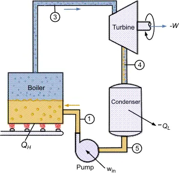
Fig-1: Rankine Cycle

The four processes of an ideal Rankine cycle are as follows:

Process 1-2: Isentropic compression in a pump. Here the working fluid is pumped from low to high pressure.

Process 2-3: Constant pressure heat addition in the boiler. In this process, the high-pressure liquid is added to the boiler and is heated at constant pressure to become a dry saturated vapour.

Process 3-4: Isentropic expansion in a turbine. The dry saturated vapour expands through the turbine resulting in the generation of power.

Process 4-1: Constant pressure heat rejection in a condenser. Wet vapour is condensed at a constant pressure to become a saturated liquid.

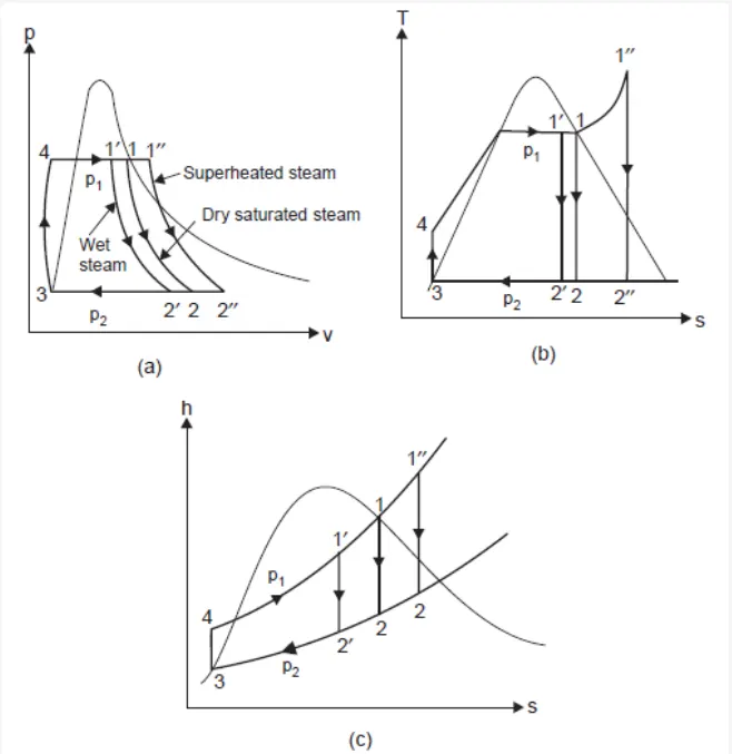
Fig-2: p-v, T-s , and h-s diagrams of Rankine Cycle

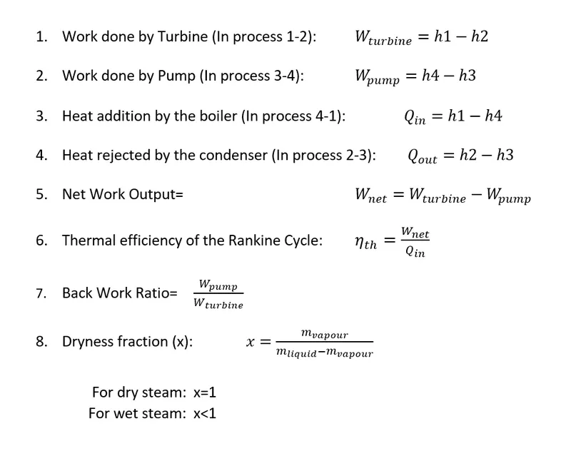
Governing Equations:

Required Inputs:

Turbine Inlet temperature = 400° C

Turbine Inlet Pressure = 30 bars

Turbine Outlet Pressure = 0.05 bars = Condenser Inlet Pressure

Matlab Code for Rankine Cycle Simulator:

clear all
close all
clc

disp('                 RANKINE CYCLE SIMULATOR              ');
disp('1-2 is an Isentropic Expansion in the Turbine.');
disp('2-3 is a Constant Pressure Heat Rejection by the Condenser.');
disp('3-4 is an Isentropic Compression in the Pump.');
disp('4-1 is a Constant Pressure Heat addition by the Boiler.');

p1=input('\nEnter the pressure at the turbine inlet (in bar)=');
T1=input('Enter the temperature at the turbine inlet (in Degree Celcius)=');
p2=input('Enter the pressure at condenser inlet (in bar)=');

%State-1
h1= XSteam('h_pT',p1,T1);   % To extract enthalpy at point-1
s1= XSteam('s_pT',p1,T1);   % To extract entropy at point-2

%State-2
s2= s1;                     % Constant isentrophic expansion
sf2= XSteam('sL_p',p2);     % Saturated liquid entropy
sg2= XSteam('sV_p',p2);     % Saturated vapour entropy
sfg= sg2-sf2;  

hf2= XSteam('hL_p',p2);     % Saturated liquid enthalpy
hg2= XSteam('hV_p',p2);     % Saturated vapour enthalpy
hfg= hg2-hf2;   

% To determine dryness fraction and enthalpy
if s2<sg2
    x2= (s2-sf2)/sfg;       % dryness fraction of wet steam(x<1)
    h2= hf2 + (x2*(hfg));   % To extract enthalpy at point-2
else
    x2=1;                   % dryness fraction of dry steam(x=1)
    h2= x2*hg2;
end

%State-3
p3=p2;                      % Constant pressure at point-3(Isobaric Process)
s3= XSteam('sL_p',p3);      % To extract entropy at point-3
h3= XSteam('hL_p',p3);      % To extract enthalpy at point-3
v3= XSteam('vL_p',p3);      % Specific volume at point-3
T3=XSteam('Tsat_p', p3);    % Saturation Temperature
T2=T3;

%State-4
s4=s3;
p4=p1;
Cv= XSteam('Cv_ps', p4, s4);   %Specific isochoric heat capacity
Cp= XSteam('Cp_ps', p4, s4);   %Specific isobaric heat capacity
g=Cp/Cv;                        % Heat Capacity Ratio
T4= T3/((p3/p4)^((g-1)/g));

Wt= h1-h2;  %Work done by turbine(Wt)
Wp= v3*(p4-p3)*100; %Work done by pump (Wp)
h4= h3 + Wp;
Wnet= Wt - Wp;  % Net work done (Wnet)
r_bw= Wp/Wt;   %Back Work Ratio

Q_in= h1-h4;    % Heat into the system
Q_out= h2-h3;   % Heat out to the system

Thermal_efficiency= (Wnet/Q_in)*100;    %Thermal Efficiency of Rankine cycle

S.S.C= 3600/Wnet;       %Specific steam consumption(S.S.C)


s5= XSteam('sL_p',p1);
s6= XSteam('sV_p',p1);
h5= XSteam('hL_p',p1);
h6= XSteam('hV_p',p1);
T6=XSteam('Tsat_p', p1);
T5=T6;

% To plot saturation curve;
T=linspace(1,375,500);     %T=Saturated Steam Temperature

for i=1:length(T)
    sf(i)= XSteam('sL_T', T(i));
    sg(i)= XSteam('sV_T', T(i));
    hf(i)= XSteam('hL_T', T(i));
    hg(i)= XSteam('hV_T', T(i));
end

%Plotting T-s diagram
figure(1)
hold on

%Plot Saturation Curve for T-s
plot(sf, T, 'color', 'b','linewidth',2)
plot(sg, T, 'color', 'r','linewidth',2)

%Plot Rankine cycle for T-s
plot([s1 s2 s3 s4 s5 s6], [T1 T2 T3 T4 T5 T6],'marker','*','linewidth',2,'color', 'k')

% To plot superheated line curve (Process 6-1)
s_1= linspace(s6,s1,500);
for j=1:length(s_1)
    T_1(j)=XSteam('T_ps',p1,s_1(j));
end
plot(s_1,T_1,'color', 'b','linewidth',2,'color', 'k')

xlabel('Entropy [kJ/kg-K]')
ylabel('Temperature[Degree Celcius]')
title('Temperature vs Entropy plot')
legend ('Saturated Liquid Curve','Saturated Vapour Curve','Rankine Cycle')
grid on
axis([0 10 0 450])

% To denote all state points
text(s1+0.1, T1, '1','color','b')
text(s2+0.1, T2, '2','color','b')
text(s3, T3-10, '3','color','b')
text(s4-0.1, T4+20, '4','color','b')
text(s5-0.1, T5+20, '5','color','b')
text(s6-0.1, T6+20, '6','color','b')

%Plotting h-s diagram
figure(2)
hold on
plot(sf, hf, 'linewidth',2,'color', 'b')
plot(sg, hg, 'linewidth',2,'color', 'r')
plot([s1 s2 s3 s4], [h1 h2 h3 h4],'marker','*','linewidth',2,'color', 'k')

h_1= linspace(h4,h5,500);
for k=1:length(h_1)
    s_2(k)=XSteam('s_ph', p1,h_1(k));
end
plot(s_2,h_1,'linewidth',2,'color', 'k')
plot([s5 s6], [h5 h6],'marker','*','linewidth',2,'color', 'k')

for l=1:length(s_1)
    h_2(l)= XSteam('h_ps',p1,s_1(l));
end

plot(s_1, h_2, 'linewidth', 2,'color', 'k')


xlabel('Entropy [kJ/kg-K]')
ylabel('Enthalpy [kJ/kg]')
title('Enthalpy vs Entropy plot')
legend ('Saturated Liquid Curve','Saturated Vapour Curve','Rankine Cycle')
grid on

% To denote all state points
text(s1+0.1,h1,'1','color', 'b')
text(s2+0.1,h2,'2','color', 'b')
text(s3,h3-50,'3','color', 'b')
text(s4,h4+150,'4','color', 'b')
text(s5,h5+100,'5','color', 'b')
text(s6,h6+100,'6','color', 'b')

%Results to display in command window
fprintf('\nRESULTS:\n');

fprintf('At State Point 1:\n');
fprintf('p1: %.2f bar\n', p1);
fprintf('T1: %.2f Degree Celcius\n', T1);
fprintf('h1: %.2f kJ/kg\n', h1);
fprintf('s1: %.2f kJ/kg-K\n\n', s1);

fprintf('At State Point 2:\n');
fprintf('p2: %.2f bar\n', p2);
fprintf('T2: %.2f Degree Celcius\n', T2);
fprintf('h2: %.2f kJ/kg\n', h2);
fprintf('s2: %.2f kJ/kg-K\n', s2);
fprintf('x2: %.2f \n\n', x2);

fprintf('At State Point 3:\n');
fprintf('p3: %.2f bar\n', p3);
fprintf('T3: %.2f Degree Celcius\n', T3);
fprintf('h3: %.2f kJ/kg\n', h3);
fprintf('s3: %.2f kJ/kg-K\n\n', s3);

fprintf('At State Point 4:\n');
fprintf('p4: %.2f bar\n', p4);
fprintf('T4: %.2f Degree Celcius\n', T4);
fprintf('h4: %.2f kJ/kg\n', h4);
fprintf('s4: %.2f kJ/kg-K\n\n', s4);

fprintf('Work done by Turbine: %.2f kJ/kg\n', Wt);
fprintf('Work done by Pump: %.2f kJ/kg\n',Wp);
fprintf('Net work output: %.2f kJ/kg\n', Wnet);
fprintf('Back Work Ratio: %.4f\n',r_bw);
fprintf('Thermal Efficiency: %.2f Percent\n',Thermal_efficiency);
fprintf('SSC: %.2f kg/kWh\n', S.S.C);

%End of program

Code Explanation:

1. Start the program with clear all, close all, and clc to clean the workspace, to close plot windows and clear command window respectively.
2. Use disp () command to print comments in command window.
3. Give the required user inputs such as p1, p2, and T1.
4. Extract the enthalpy, entropy, pressure and temperatures at state points- 1, 2,3, 4 from function (XSteam.m). Also calculates work done by pump and turbine, net work output, back work ratio, heat addition, heat rejection, thermal efficiency, and specific steam consumption.
5. Now define the range of temperature using linspace command to plot the graph. The range of temperature is taken from steam table (Min. temp-0.01 & Max. 374.14).
6. Now define the entropy and enthalpy values for liquid and vapour lines.
7. Now plot the T-s and h-s graphs and provide the labelling, title, legends, and marking the state points.
8. Now display all the state points values and other results in command window using fprintf() command.
9. End

Output (Plots):

Plot-1: T-s diagram of Rankine Cycle

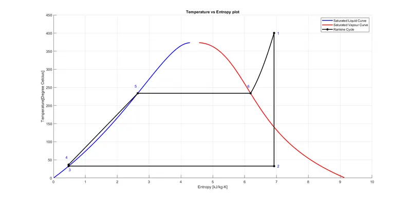
Plot-2: h-s diagram of Rankine Cycle

Output (Command Window):

                 RANKINE CYCLE SIMULATOR              
1-2 is an Isentropic Expansion in the Turbine.
2-3 is a Constant Pressure Heat Rejection by the Condenser.
3-4 is an Isentropic Compression in the Pump.
4-1 is a Constant Pressure Heat addition by the Boiler.

Enter the pressure at the turbine inlet (in bar)=30
Enter the temperature at the turbine inlet (in Degree Celcius)=400
Enter the pressure at condenser inlet (in bar)=0.05

RESULTS:
At State Point 1:
p1: 30.00 bar
T1: 400.00 Degree Celcius
h1: 3231.57 kJ/kg
s1: 6.92 kJ/kg-K

At State Point 2:
p2: 0.05 bar
T2: 32.88 Degree Celcius
h2: 2110.71 kJ/kg
s2: 6.92 kJ/kg-K
x2: 0.81 

At State Point 3:
p3: 0.05 bar
T3: 32.88 Degree Celcius
h3: 137.77 kJ/kg
s3: 0.48 kJ/kg-K

At State Point 4:
p4: 30.00 bar
T4: 36.94 Degree Celcius
h4: 140.78 kJ/kg
s4: 0.48 kJ/kg-K

Work done by Turbine: 1120.86 kJ/kg
Work done by Pump: 3.01 kJ/kg
Net work output: 1117.85 kJ/kg
Back Work Ratio: 0.0027
Thermal Efficiency: 36.17 Percent
SSC: 3.22 kg/kWh
>> 

Errors:

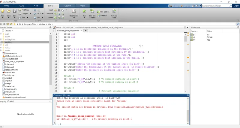
1. The particular error came beacuse mistakely I put the wrong function name (Xsteam.m) in the code. After putting the correct function name (XSteam) the error completely removed. The screenshot of the error display is attached below.

Conclusions:

1. Successfully created a Rankine Cycle Simulator using MATLAB code and calculate all the state points of the Rankine Cycle based on user inputs.
2. Plots all the corresponding T-s and h-s plots for the given set of inputs. Title, axes, labels, and legends were also shown in the both plots.
3. Calculate the Net work Output and Back Work Ratio and display those in command window display.
4. References of all study materials are added in reference section of the answer box.

References:

https://en.wikipedia.org/wiki/Enthalpy%E2%80%93entropy_chart

https://en.wikipedia.org/wiki/Rankine_cycle

https://in.mathworks.com/matlabcentral/fileexchange/9817-x-steam-thermodynamic-properties-of-water-and-steam

https://www.youtube.com/watch?v=gAGezS-Ngk4

https://www.slideshare.net/Lahiru_Dilshan/thermodynamic-assignment-2

Book- Steam and Gas Turbines and Power Plant Engineering