Solving second order ODEs

AIM: Write a program that solves the ODE for simple pendulum mathematical model and simulate the pendulum motion.

GOVERNING EQUATIONS:

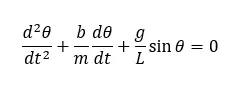
Where,

b= Damping coefficient

m= Mass of the bob (in kg)

g= Acceleration due to gravity (in m/s²)

L= Length of the pendulum (in meters)

Theory:

What is Simple Pendulum?

A point mass attached to a light inextensible string and suspended from fixed support is called a simple pendulum. The vertical line passing through the fixed support is the mean position of a simple pendulum. The vertical distance between the point of suspension and the centre of mass of the suspended body (when it is in mean position) is called the length of the simple pendulum denoted by L.

A simple pendulum is a mechanical arrangement that demonstrates periodic motion. The simple pendulum comprises of a small bob of mass ‘m’ suspended by a thin string secured to a platform at its upper end of length L.

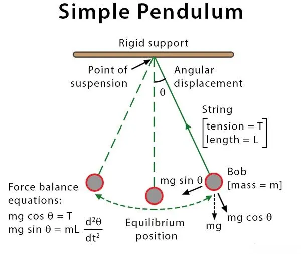
Fig.1: Simple Pendulum

Important Terms

• The oscillatory motion of a simple pendulum:Oscillatory motion is defined as the to and fro motion of the pendulum in a periodic fashion and the centre point of oscillation known as equilibrium position.
• The time period of a simple pendulum:It is defined as the time taken by the pendulum to finish one full oscillation and is denoted by “T”.
• The amplitude of simple pendulum:It is defined as the distance travelled by the pendulum from the equilibrium position to one side.
• Length of a simple pendulum:It is defined as the distance between the point of suspension to the centre of the bob and is denoted by “L”.
• Displacement (x): Distance traveled by the pendulum bob from the equilibrium position to one side. The angle described by the pendulum with an imaginary axis at the equilibrium position is called the angular displacement (θ).

Assumptions:

• There is negligible friction from the air and the system.
• The arm of the pendulum does not bend or compress and is massless.
• The pendulum swings in a perfect plane.
• Gravity remains constant.

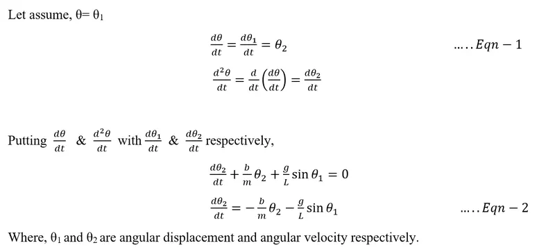
Workflow:

• Matlab can solve linear differential equations much easily. Hence, we will convert the pendulum equation to linear form and then define it in Matlab code.
• When we convert the pendulum’s second order differential equation to linear form, we get two equations-1 & 2.

Matlab Code:

Function

function [dtheta_dt]=ode_function_for_pendulum(t, theta,b,g,l,m)
theta1= theta(1);
theta2= theta(2);
dtheta1_dt= theta2 ;
dtheta2_dt=-(b/m)*theta2 - (g/l)*sin(theta1);
dtheta_dt= [dtheta1_dt;dtheta2_dt];
end

Main Code

%Write a program that solves the ODE and simulate the pendulum motion.
clear all
close all
clc

%Inputs (data was reterived from this challange question)
b=0.05;  %damping co-efficient= b
g=9.81;  %gravitational acceleration= g(m/s^2)
l=1;     %length of pendulum= l (m)
m=0.1;   %mass=m (kg)

%Initial conditions
theta_0= [0;3]; %Here, angular displacement=0, and angular displacement=3 rad/s at time t=0.

%time points
t_span= linspace(0,20,500);  %Here, time of simulation is from 0-20 second.

%solve ODE
[t,results]= ode45(@(t,theta)ode_function_for_pendulum(t, theta,b,g,l,m),t_span,theta_0);

figure(1)       %To plot the Angular displacement and Angular velocity graph of pendulum
hold on
plot(t,results(:,1))
plot(t,results(:,2))

xlabel('Time (Seconds)')
ylabel('Plot')
legend('Displacement', 'Velocity')
title('Variation of Angular displacement and Angular Velocity with time')
grid on

% FOR loop 
ct=1; %count for the iteration
for i=1:500
    x0=0;                   %first end of pendulum, x-coordinate
    y0=0;                   %first end of pendulum, y-coordinate
    
   x1=l*sin(results(i,1));  %Second end of pendulum, x-coordinate
   y1=-l*cos(results(i,1)); %Second end of pendulum, y-coordinate
   
  figure(2)     %Plot to simulate the motion of simple pendulum
  plot([-0.5,0.5],[0,0],'linewidth',3); % To plot the rigid support for pendulum
  hold on
  plot([x0,x1],[y0,y1],'linewidth',2);  % To plot the pendulum string
  hold on
  plot(x1,y1,'marker','O', 'linewidth',8); % To plot the pendulum bob
  hold on
  axis([-1 1 -1.5 0.5]);                    % To define axis limit of graph area
  title('Simulation of Motion of Simple Pendulum')
  grid on
  pause(0.01)
  hold off
  P(ct)=getframe(gcf);
  ct=ct+1;
end
  
  
movie(P)% Generating movie file from frames
videofile=VideoWriter('Pendulum_animation.avi','uncompressed AVI'); %Saving the movie in disk as .AVI format 
open(videofile)%Opening of movie file
writeVideo(videofile,P)%writing of movie file
close(videofile)%closing of movie file

%close of program

Output:

See attatchment and youtube link for graph and animation of simple pendulum.

Youtube link for simulation vidoe of pendulum:

https://youtu.be/W8AgQwOaJTQ

Note:

1. No error was faced in executing and simulation of progam.

References:

1. Simple Pendulum - Time Period, Derivation, and Physical Pendulum (byjus.com)

2.Simple Pendulum: Theory, Diagram, and Formula. (sciencefacts.net)