Project 1 - Parsing NASA thermodynamic data
Aim: The aim of this challenge is to learn and understand the parsing of data (NASA thermodynamic) and extract the coefficients to calculate the thermodynamic properties of each individual species.
Governing Equation:
The equation to calculate the Specific Heat, Enthalpy and Entropy of each species is given below. The equation is already provided in this challenge.

Objectives:
- Write a function that extracts the 14 co-efficients and calculates the enthalpy, entropy, and specific heats for all the species in the data file.
- Calculate the molecular weight of each species and display it in the command window.
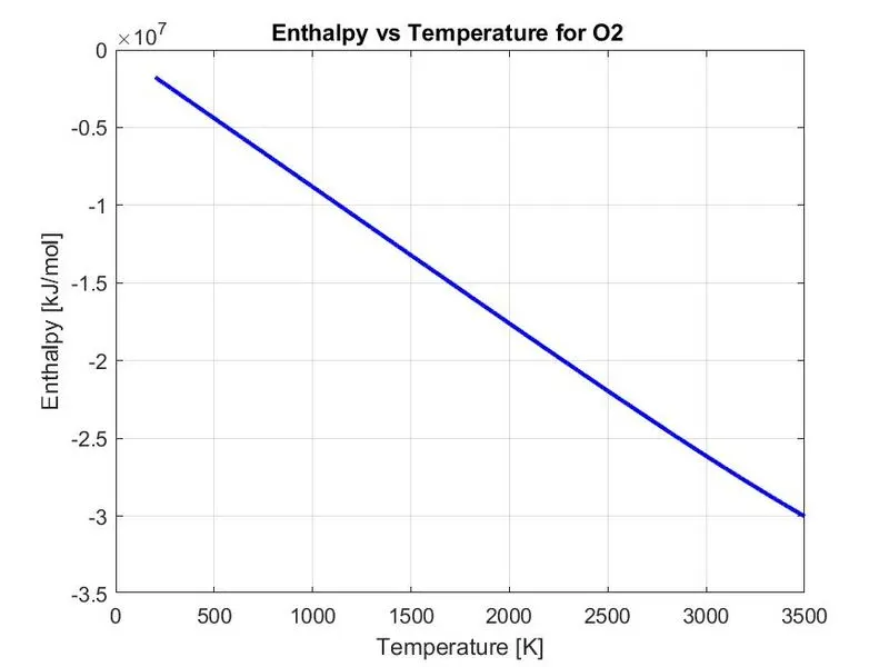
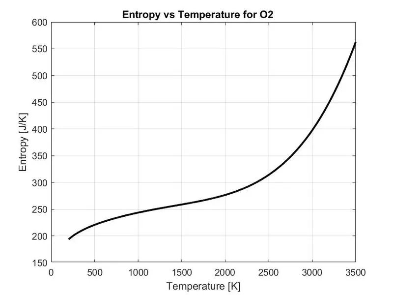
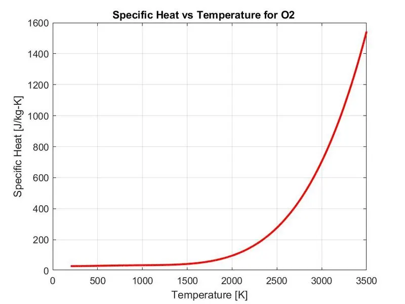
- Plot the Cp, Enthalpy, and Entropy for the local temperature range (low temperature: high temperature) specific for each species.
- Save the plots as images with appropriate names and dump them in separate folders for each species with a suitable name. All these should be generated automatically.
- The main program that you will submit will just take the "THERMO.dat" file as an input and generate Cp, H, and S-plots.
- Please write a detailed report to describe your logic.
Theory:
File Parsing:
Parse essentially means to “resolve (a sentence) into its component parts and describe their syntactic roles”. In computing, Parsing is an act of splitting a string or a text. In this method of parsing the file or other input into a piece of data that can be easily stored or manipulated. By doing this we are going to split a string into parts then recognizing the parts to convert it into something simpler than a string.
NASA Thermodynamic Data:
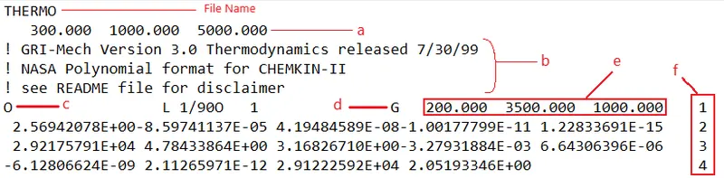
NASA thermodynamic data which is THERMO.dat file in which there are temperature ranges and 53 species are given in these data and each species contains 14 coefficients and temperature ranges and we have to parse 14 coefficients to find Specific Heat, Entropy, Enthalpy using the governing equation. In the challenge, we have to extract the necessary information from the file to calculate the properties of the species and plot them. This process of extracting information from the file is called File Parsing.
File- THERMO.dat
Where,
- First line “THERMO” is the file name of or say it is heading of the data.
- ‘a’ represents as the ‘Global Temperature Ranges’.
- ‘b’ represents as the ‘Comments’.
- ‘c’ represents as ‘Species Name’.
- ‘d’ represents as physical state of species. Where, S- Solid, L-Liquid, G-Gas.
- ‘e’ represents as ‘Species Temperature Ranges’.
- ‘f’ represents as the three lines where coefficients are organised to calculate Enthalpy, Entropy, and Specific Heat.
Matlab Code:
Function (To calculate molecular weight of species):
%Function to calculate molecular mass of species.

function M= molecular_weight(species_name)
elements= ['H', 'C', 'N', 'O', 'A'];
atomic_weight= [1 12 14 16 40];
M=0;

for i=1:length(species_name)
    for j=1:length(elements)
        if strcmp(species_name(i),elements(j))      % To compare strings "strcmp" is used.
            M= M+ atomic_weight(j);
            x=j;
        end
    end
    n=str2double(species_name(i));

    if n>1
        M= M +(atomic_weight(x)*(n-1));
    end
end
end
Main Program:
clear all
close all
clc

file=fopen('THERMO.dat','r');    % To open the file and read the THERMO data.
line1=fgetl(file);              % To getting the file name of data from first line.
line2=fgetl(file);              % To getting the temperature values from the second line.

% To getting the comments from the next three line.
comment_1=fgetl(file);
comment_2=fgetl(file);
comment_3=fgetl(file);

A= strsplit(line2,' ');                % Splitting the second line to extract the global temperature values.
global_low_temp= str2double(A{2});     % Global low temperature.
global_medium_temp= str2double(A{3});  % Global medium temperature.
global_high_temp= str2double(A{4});    % Global high temperature.

% To extract the individual species information.
for i=1:53                          % For total 53 individual species.
    species=fgetl(file);

    T1= strfind(species,'.');

    local_low_temp= str2double(species(T1(1)-3:T1(1)+3));      % Local low temperature.
    local_high_temp= str2double(species(T1(2)-4:T1(2)+3));     % Local high temperature.
    local_medium_temp= str2double(T1(3)-4:T1(3)+3);            % Local medium temperature.

    species_name= species(1:6);     % To read the species name (longest species has 6 alphabets).

    l1=fgetl(file);     % Getting first line of species
    l2=fgetl(file);     % Getting second line of species
    l3=fgetl(file);     % Getting third line of species

    % Extracting the constants a1 to a5 from 1st species line using "E" as
    % locate the position
    position_1= strfind(l1,'E');
    a1=str2double(l1(1:position_1(1)+3));
    a2=str2double(l1(1:position_1(1)+4:position_1(2)+3));
    a3=str2double(l1(1:position_1(2)+4:position_1(3)+3));
    a4=str2double(l1(1:position_1(3)+4:position_1(4)+3));
    a5=str2double(l1(1:position_1(4)+4:position_1(5)+3));

    % Extracting the constants a5 to a10 from 2nd species line using "E" as
    % locate the position
    position_2= strfind(l2,'E');
    a6=str2double(l2(1:position_2(1)+3));
    a7=str2double(l2(position_2(1)+4:position_2(2)+3));
    a8=str2double(l2(position_2(2)+4:position_2(3)+3));
    a9=str2double(l2(position_2(3)+4:position_2(4)+3));
    a10=str2double(l2(position_2(4)+4:position_2(5)+3));

    % Extracting the constants a11 to a14 from 3rd species line using "E" as
    % locate the position
    position_3= strfind(l3,'E');
    a11=str2double(l3(1:position_3(1)+3));
    a12=str2double(l3(position_3(1)+4:position_3(2)+3));
    a13=str2double(l3(position_3(2)+4:position_3(3)+3));
    a14=str2double(l3(position_3(3)+4:position_3(4)+3));


    R=8.314;  % Universal gas constant(J/mol-k)
    T=local_low_temp:local_high_temp; % Taking temperature value between local lowand high temperature range


    % To calculate the Specific Heat (Cp), Enthalpy (H), and Entropy (S)

    if (T>local_medium_temp)
        Cp= R*(a1+(a2*T) + (a3*(T.^2)) + (a4*(T.^3)) + (a5*(T.^4)));

        H= R*T.*(a1 + ((a2*T)/2) + (a3*(T.^2)/3) + (a4*(T.^3)/4) + (a5*(T.^4)/5) + a6);

        S= R*((a1.*log(T)) + (a2*T) + (a3*(T.^2)/2) + (a4*(T.^3)/3) + (a5*(T.^4)/4) + a7);

    else
        Cp= R*(a8+(a9*T) + (a10*(T.^2)) + (a11*(T.^3)) + (a12*(T.^4)));

        H= R*T.*(a8 + ((a9*T)/2) + (a10*(T.^2)/3) + (a11*(T.^3)/4) + (a12*(T.^4)/5) + a13);

        S= R*((a8.*log(T)) + (a9*T) + (a10*(T.^2)/2) + (a11*(T.^3)/3) + (a12*(T.^4)/4) + a14);
    end


    % Plotting of figures
    figure(1)
    plot(T,Cp,'color','r','linewidth',2);
    xlabel('Temperature [K]')
    ylabel('Specific Heat [J/kg-K]')
    title(sprintf('Specific Heat vs Temperature for %s',species_name));
    grid on

    figure(2)
    plot(T,H,'color','b','linewidth',2)
    xlabel('Temperature [K]')
    ylabel('Enthalpy [kJ/mol]')
    title(sprintf('Enthalpy vs Temperature for %s',species_name));
    grid on

    figure(3)
    plot(T,S,'color','k','linewidth',2)
    xlabel('Temperature [K]')
    ylabel('Entropy [J/K]')
    title(sprintf('Entropy vs Temperature for %s',species_name));
    grid on

    cd('D:\Skill-Lync Course\Projects\NASA Thermodynamic\Generated Plots')    % Changing the file path to save the plots.
    mkdir(species_name);        % Creating file directory for each species.
    warning('off','MATLAB:MKDIR:DirectoryExists');
    cd(species_name);           % To create the species with species name.

    % To save the plots in allocated folder.
    saveas(1,'Specific_Heat.jpg');
    saveas(2,'Enthalpy.jpg');
    saveas(3,'Entropy.jpg');

    cd('D:\Skill-Lync Course\Projects\NASA Thermodynamic');    % To change folder again to calculate molecular weight of species.
    mol_weight=molecular_weight(species_name);       % To calculate molecular weight of each species from function.
    W= sprintf('The molecular weight of %s is %.2f', species_name, mol_weight);    % To print molecular weight of species.
    disp(W)        % To display the print data in the command window.

end
fclose(file);        % To close the file.

% End of program.
Output Plots:
Species-O2:
Species-N2:
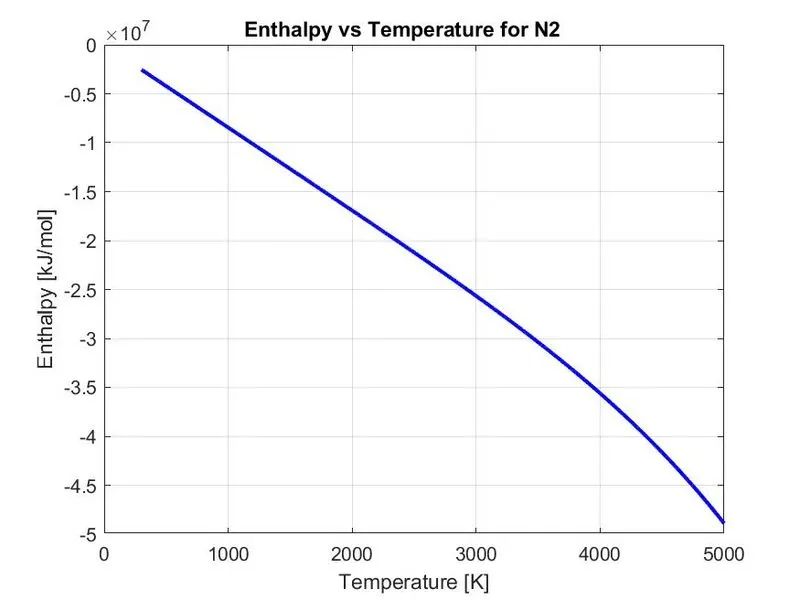
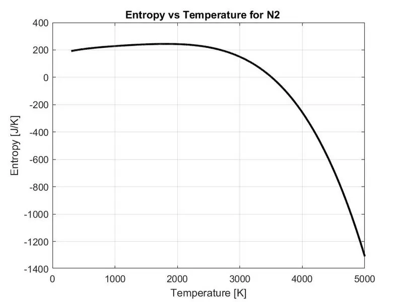
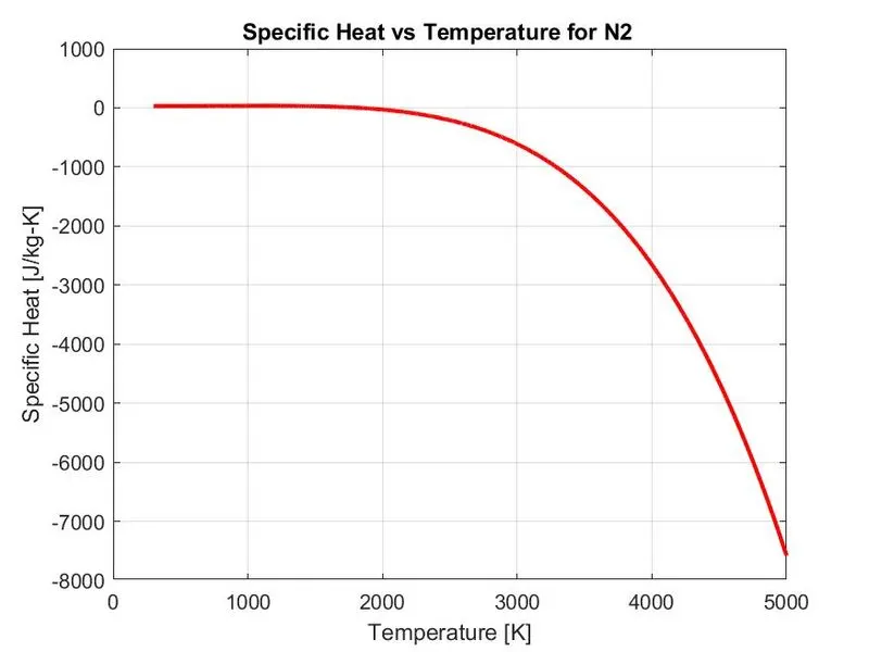
Species-CO2:
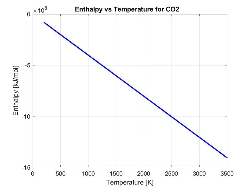
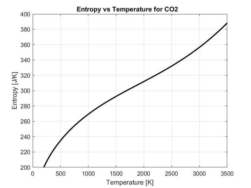
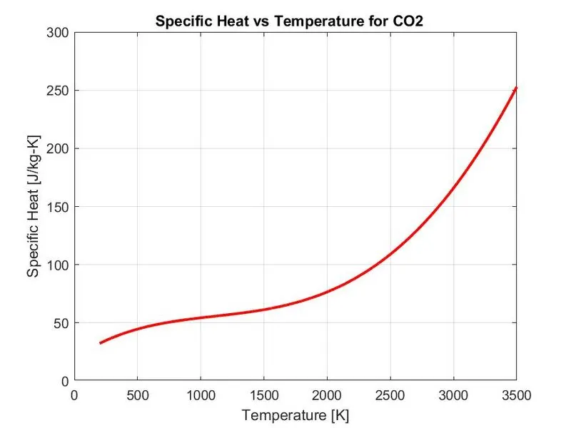
Output (Command Window):
The molecular weight of O      is 16.00
The molecular weight of O2     is 32.00
The molecular weight of H      is 1.00
The molecular weight of H2     is 2.00
The molecular weight of OH     is 17.00
The molecular weight of H2O    is 18.00
The molecular weight of HO2    is 33.00
The molecular weight of H2O2   is 34.00
The molecular weight of C      is 12.00
The molecular weight of CH     is 13.00
The molecular weight of CH2    is 14.00
The molecular weight of CH2(S) is 14.00
The molecular weight of CH3    is 15.00
The molecular weight of CH4    is 16.00
The molecular weight of CO     is 28.00
The molecular weight of CO2    is 44.00
The molecular weight of HCO    is 29.00
The molecular weight of CH2O   is 30.00
The molecular weight of CH2OH  is 31.00
The molecular weight of CH3O   is 31.00
The molecular weight of CH3OH  is 32.00
The molecular weight of C2H    is 25.00
The molecular weight of C2H2   is 26.00
The molecular weight of C2H3   is 27.00
The molecular weight of C2H4   is 28.00
The molecular weight of C2H5   is 29.00
The molecular weight of C2H6   is 30.00
The molecular weight of CH2CO  is 42.00
The molecular weight of HCCO   is 41.00
The molecular weight of HCCOH  is 42.00
The molecular weight of H2CN   is 28.00
The molecular weight of HCN    is 27.00
The molecular weight of HNO    is 31.00
The molecular weight of N      is 14.00
The molecular weight of NNH    is 29.00
The molecular weight of N2O    is 44.00
The molecular weight of NH     is 15.00
The molecular weight of NH2    is 16.00
The molecular weight of NH3    is 17.00
The molecular weight of NO     is 30.00
The molecular weight of NO2    is 46.00
The molecular weight of HCNO   is 43.00
The molecular weight of HOCN   is 43.00
The molecular weight of HNCO   is 43.00
The molecular weight of NCO    is 42.00
The molecular weight of CN     is 26.00
The molecular weight of HCNN   is 41.00
The molecular weight of N2     is 28.00
The molecular weight of AR     is 40.00
The molecular weight of C3H8   is 44.00
The molecular weight of C3H7   is 43.00
The molecular weight of CH3CHO is 44.00
The molecular weight of CH2CHO is 43.00
>>
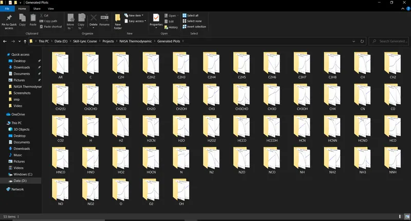
Screenshot of the window where all the folders are saved:
Code Explanation (Main Program):
- Start the program with “clear all”, “close all”, “clc” to clears the workspace, close all the figure windows and clears the command window.
- By using “fopen” command we open our file names as “THERMO.dat” and use “r” to read that particular file. A variable “file” is used to save that open data.
- Then by using “fgetl” command to read every single line of the file. From the first line and second line of data is called to store the file name and temperature values. For first line “line1” and for second line “line2” is used to store the called data.
- Now using “strsplit” command to split the data. Split data is further stored in a variable named as “A”.
- Now global temperature values are stored in variable by using “str2double” command. “str2double” command is used to convert text (string) into numerical value.
- After assigning global low, medium, and high temperature values we have to find local low, medium, and high temperature values. For that “for loop” command is used. In the loop, “strfind” is again used to find the local temperature values. To find the temperature values we need a reference point. Here reference point was decimal value (.). After that string is converted into double precision numeric value using “str2double” and that numeric values are stored in “local_low_temp”, “local_high_temp”, and “local_medium_temp” variables.
- Now the species names are read and stored in “species_name” variable.
- Now for getting the value of the coefficients for each species firstly “fgetl” is used for reading the first coefficients line and storing the data. Then using “strfind” command for locating ‘E’ and then places are added to get the whole value and is stored in “position_1”.
- After that it is converted into a double precision value using “str2double” command and then the numeric value is stored. Then same process is performed for line 2 (l1), line 3 (l2), and line 4 (l3). The variables in which the numeric values were stored are: a1, a2, a3, a4, a5, a6, a7, a8, a9, a10, a11, a12, a13, a14.
- Now the local temperature values are put in variable “T”. the temperature values are equally distributed (in a series and difference was 1) in between 200 to 3500. Example- 200, 201, 202, 203, . . . . . .., 3500.
- Now the equations were written to calculate specific heat, enthalpy, entropy of species and stored in Cp, H, S respectively.
- After that to plotting and then saving those plots in separate folder, “mkdir” anew folder is created by species name and its name is changed to the species name using “cd” command.
- To plot all graph in sperate window “figure( )” command is used. After that x-label, y-label, and title of plot is provided.
- To save the plots in allocated folder “saveas” command is used with file name and its extension.
- To calculate the molecular weight of the species, the function called “molecular_weight(species_name)” is called and stored in “mol_weight”. For display that in command window “disp( )” command is used.
- At the last step “fclose” command is used after the loop end to close the file. And the program is ended.
Code Explanation (Function)
- A function is created by giving a name to it and then save it to “molecular _weight”.
- Now element and atomic weight is provided and stored in “elements” and “atomic_weight” respectively.
- After that “for” loop is used for the species which has a length of six, another loop is used to get "elements".
- Using “strcmp” command is used to compare strings- “species_name” and “elements”.
- Now the molecular weight is calculated by the written formula (see code) and the value is stored in M.
Error:
In this challenge, I encountered some errors while writing and executing the program code. The details of those errors are discussed below:
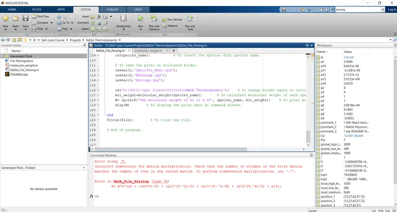
1. The first error was because of a mistake in my equation. The mistake was that I forget to put the element-wise operator in variable "H". By putting "." I removed that error. Here I attached the screenshot of that error.
2. The second error was a warning- "Warning: Directory already exists". To remove this error the following code is written:
warning('off','MATLAB:MKDIR:DirectoryExists');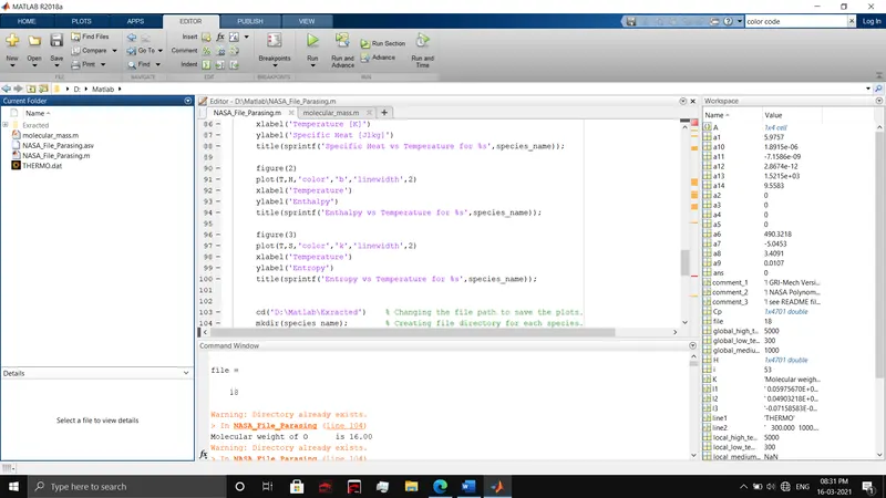
Conclusion:
- The program was run successfully and completed parsing of NASA Thermodynamic data.
- Molecular weight is calculated for all species and displayed in command window.
- Plots of Specific Heat, Entropy, and Enthalpy for all species have generated and saved in a separate folder named according to species.
- All the attachments and code explanations are provided in the answer box.
- Zipped file of all generated plots is attached here (see the attachment section).
References:
- https://skill-lync.com/projects/File-Parsing-and-Data-Analysis-in-Python-Part-I-Interactive-Parsing-and-Data-Visualisation-24878#:~:text=Parse%20essentially%20means%20to%20%27%27,as%20per%20the%20formal%20grammar.
- https://www.mathworks.com/help/releases/R2018a/matlab/ref/mkdir.html
- https://www.mathworks.com/help/releases/R2018a/matlab/ref/cd.html
- https://www.mathworks.com/help/releases/R2018a/matlab/ref/strcmp.html
Note: I have attached all the images in the attachment section. These images are the same as those given in the answer box.