Week-4 Challenge WOT Condition Part-2

1. What is the difference between mapped and dynamic model of engine, motor and generator? How can you change model type?

Ans:

Mapped model:

1. In this, model data is used for operation and simulation. This model data can be obtained from lookup table.
2. Time for simulation will be very less as it use look up table data.
3. Accutacy of the system is very less compare to Dyanamic model.
4. Because it will not take real time data.

Dyanamic model:

1. Here it understand the behaviour of real time elements and behaves accordingly.
2. Here we will get detail analysis of particular element.
3. Time for simulation is more as each and every element Performance is caliculated.
4. Results obatained are more accurate compare to Mapped model.

Engine Model:

Mapped model: Engine performance is simulated with data present in look up table which are entered in array format.

Dynamic Model: Engine performance is simulated with specfications of engine.

Generator Model:

Mapped model: Torque ,speed, maximum efficiency are taken from look up table.

Dynamic Model: The actual details are considered and caliculated.

Motor Model:

Mapped model: Torque ,speed, maximum efficiency are taken from look up table.

Dynamic Model: The actual details are considered and caliculated.

Changing Model from Mapped to Dyanamic model:

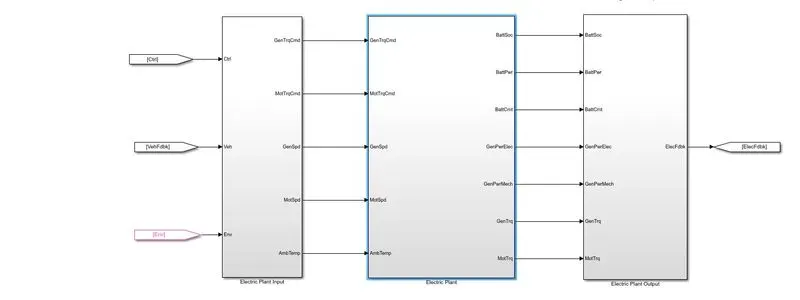
Select electric plant in above figure

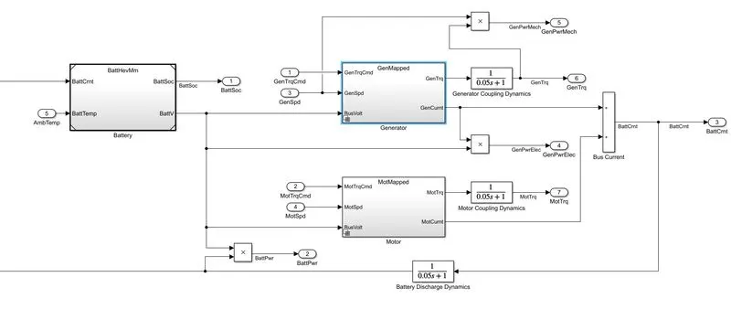
Right Click on Genertaor or Motor Model to change from dynamic to mapped or vice versa.

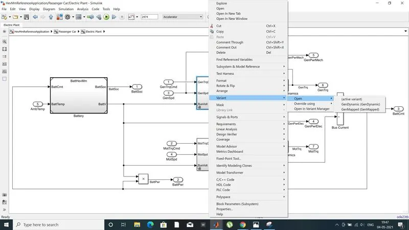
After right clicking on mouse select varian as shown in above figure, then it can changed to dyanamic or mapped model.

2. How does the model calculate miles per gallon? Which factors are considered to model fuel flow?

Ans:

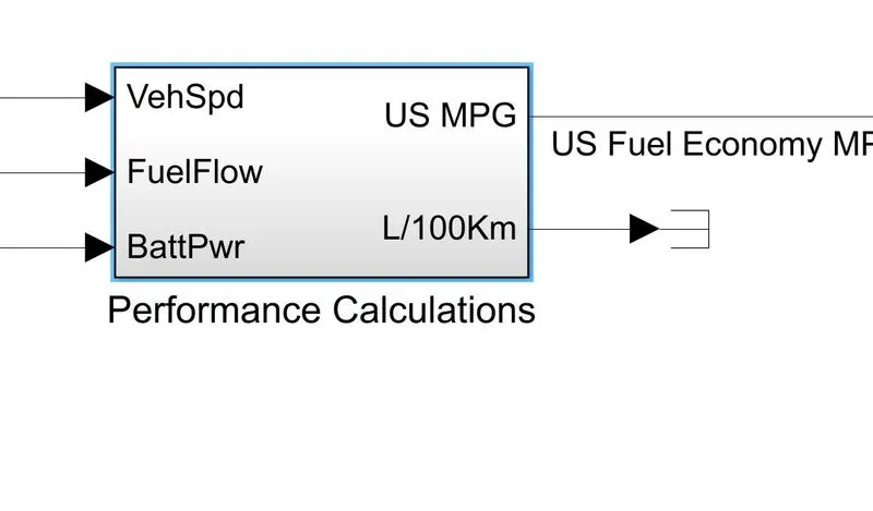
Factors are considered to fuel flow:

1: Vechicle speed

2: Fuel Flow

3: Battery power

Procedure to calculate the fuel flow:

Battery Power:

Generally batteries are required to store an electrical energy. This energy is supplied to Vechicle.

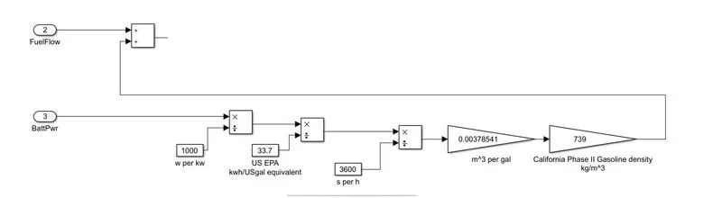
Conversion Involved in Battery power into m^3 per gallon

1. Battery power obtained in watts is converted into Kw by dividing 1000.
2. After converting into kw, divide by 33.7 so it is converted into US EPA.
3. Again divide by 3600 so this value is converted per hour
4. Multiply above obtained with 0.00378541, therefore it is converted into m^3 per gallon.

Fuel Flow and battery Power:

1. Battery power obtained in m^3 and fuel flow are added using adder block.
2. This are Intergrted over a period of time using Integrator block.
3. The value obtained is in m^3. To convert into US gallon ,multiply with 264.72.

Vechicle speed:

1. Vechicle speed is converted to distance coverge using intergrator block
2. Distance obtained is in meters.To convert into miles,Frist convert the value per 100km dividing by 1/100/1000.
3. Know value obtained is in per 100km.
4. By multiplying above value with 0.000621 we will get value in miles.

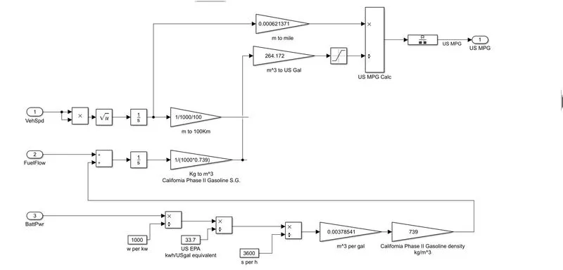
Procedure for Calculating miles per gallon.

1. Vechicle speed which is converted into miles as explained above is divide by sum of fuel flow and battery power which are obtained as US gallon.
2. Distance is in miles and fuel power in us gallons are divided for calculating miles per gallon as shown in above figure.

3.Run the HEV ReferenceApplication with WOT drive cycle. Change the grade and wind velocity in the environment block. Comment on the results.

Ans:

Type autoblkHevStart in command window of Matlab. The HEV Reference Application file will be opened as shown below.

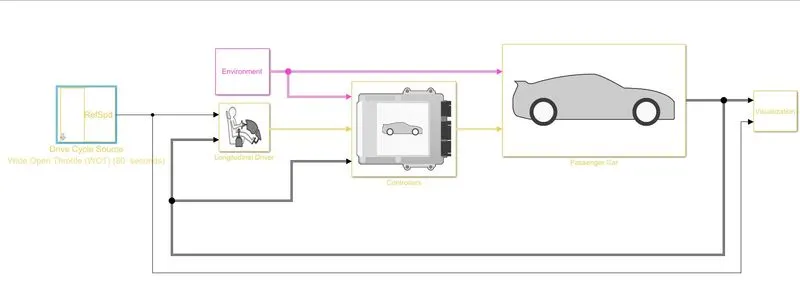
Wot condition without changes:

Change Drive cycle to WOT with 80 seconds as simulation time. Normal Reference speed is taken as 30 and vechile start deceleration at 50 sec.

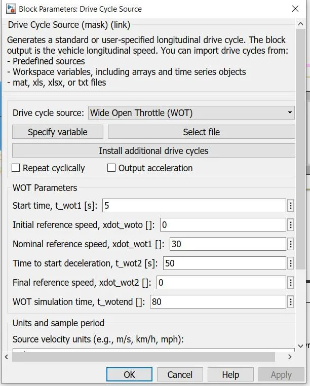
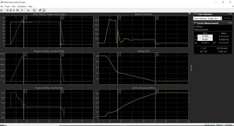
The HEV model is similuted with above WOT drive cycle values.The following results are obtained.

Analysing the Results:

Plot 1:Trace velocity , Target veclocity with respect to time.

At T= 16.985sec trace velocity reaches target vecloity. This delay happens due to internal behaviour of the system. To reduce this delay, PID controller can be added.

At T=50.622 velocity of vechicle decreses as per input command. It takes extra 6 secs for velocity becomes zero.

Plot 2: Engine speed, motor speed ,Generator speed.

This plot shows how Engine speed, motor speed and Generator speed are varied with respect to time. Speed reaches nearly 8000rpm at steady state. At peakovershoot speed reaches nearly 9000 rpm for small duration.

Plot 3:Engine Torque, motor Torque,Generator Torque.

As velocity increases Torque of this engine,motor,generator increases. when speed reches it traget speed , torque this will be reduced as shown in plot. At=50.622 sec Torque reaches to negative value as now vechicle is now operating in regenerative mode.

Plot 4: Battery current

At starting battery current is maximum till vechicle reches its actual speed. At T=16.985 velocity reaches its target value then battery current reaches to minimum value.

At T=50.622 sec motor is operating in regenerative mode, therofore battery current changes its direction.

Plot 5 : Battery SOC

From T=16.985 to 50.622, battery State of charge reaches to 68% From 80%.

Plot 6:

This plot shows US fuel economy with respect to time. As distance increases Fuel economy increases . In this plot fuel economy reaches to 50 from 0.

Wot condition with changes in wind and grade:

change the grade and wind values as shown below.

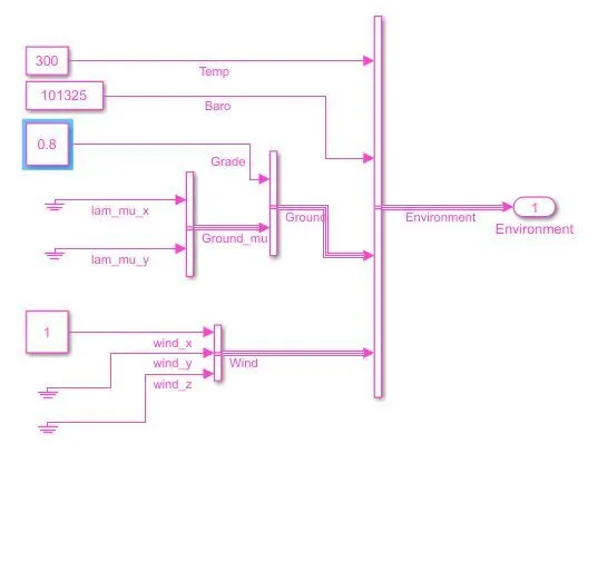
In above figure wind values is taken as 1 and grade value is taken as 0.8 and model is simulated with this changes.Follwing results are obtained.

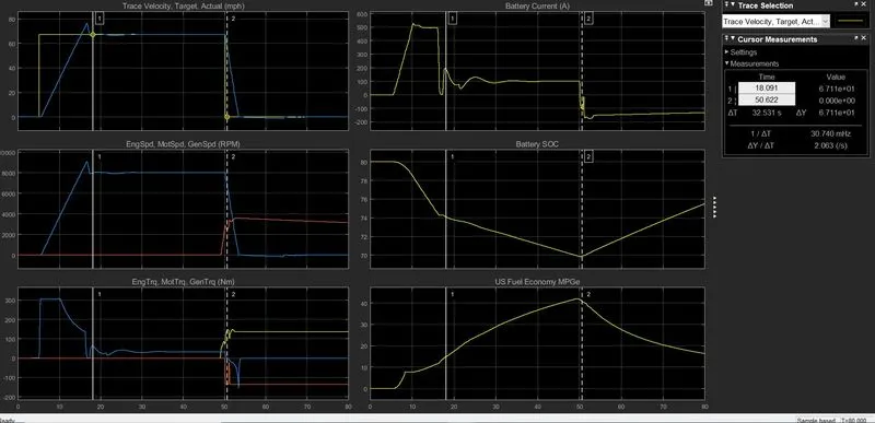
Analysing the Results:

Plot 1:Trace velocity , Target veclocity with respect to time.

At T= 18.091 sec trace velocity reaches target vecloity. This delay happens due to internal behaviour of the system. To reduce this delay, PID controller can be added.

At T=50.622 velocity of vechicle decreses as per input command. It takes extra 6 secs for velocity becomes zero.

Plot 2: Engine speed, motor speed ,Generator speed.

This plot shows how Engine speed, motor speed and Generator speed are varied with respect to time. Speed reaches nearly 10000rpm at steady state. At peakovershoot speed reaches nearly11000rpm for small duration.

Plot 3:Engine Torque, motor Torque,Generator Torque.

As velocity increases Torque of this engine,motor,generator increases. when speed reches it traget speed , torque this will be reduced as shown in plot. At=50.622 sec Torque reaches to negative value as now vechicle is now operating in regenerative mode.

Plot 4: Battery current

At starting battery current is maximum till vechicle reches its actual speed. At T=18.091 velocity reaches its target value then battery current reaches to minimum value.

At T=50.622 sec motor is operating in regenerative mode, therofore battery current changes its direction.

Plot 5 : Battery SOC

From T=18.091 to 50.622, battery State of charge reaches to 70% From 80%. Battery usage is less because due to garde and wind velocity.

Plot 6:US fuel economy

This plot shows US fuel economy with respect to time. As distance increases Fuel economy increases . In this plot fuel economy reaches to 40 from 0.

S.no	Parmeters	WOT with out changes	Wot with changes
1	Velocity time	T=16.985	T=18.091
2	Engine speed, motor speed ,Generator speed	8000rpm	9000rpm
3	Battery current	2nd peak over shoot I=280A	2nd peak over shoot I=200A
4	Battery SOC	80 to 68	80 to 70
5	US fuel economy	0 to 50	0 to 40

4. Keeping all other parameters same, compare the simulated results of hybrid and pure electric powertrains.

Ans

Type autoblkEvStart in command window of Matlab. The HEV Reference Application file will be opened as shown below.

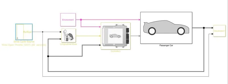
Wot condition with changes:

Change Drive cycle to WOT with 80 seconds as simulation time. Normal Reference speed is taken as 30 and vechile start deceleration at 50 sec.

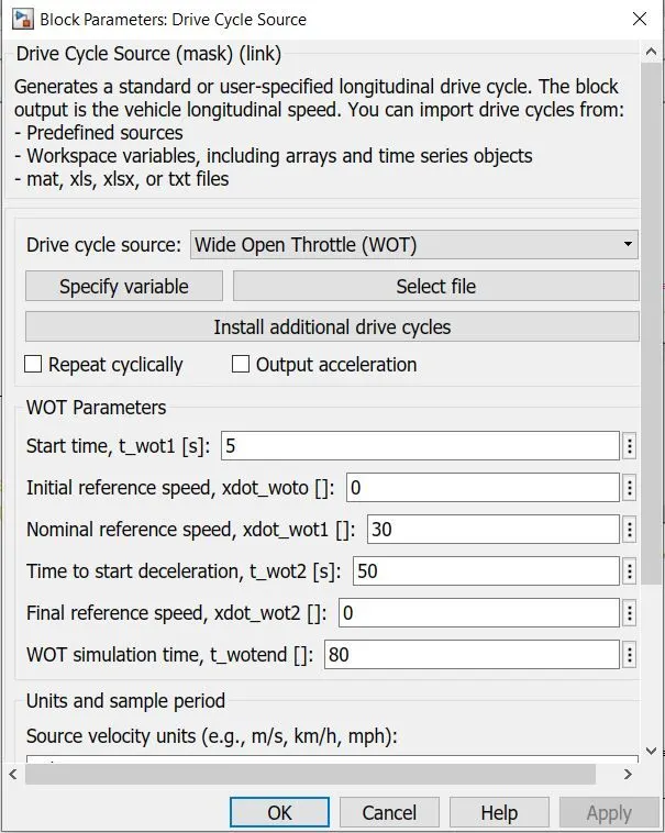
change the grade and wind values as shown below.

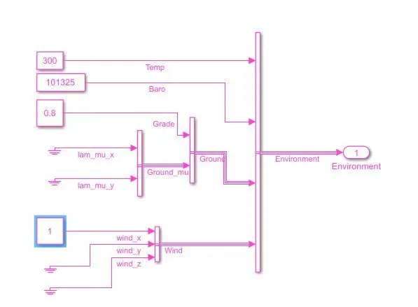
In above figure wind values is taken as 1 and grade value is taken as 0.8 and model is simulated with this changes.Follwing results are obtained.

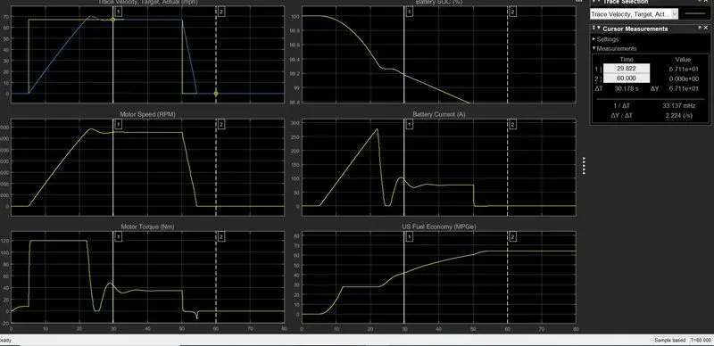
Analysing the Results:

Plot 1:Trace velocity , Target veclocity with respect to time.

At T= 29.8 sec trace velocity reaches target vecloity. This delay happens due to internal behaviour of the system. To reduce this delay, PID controller can be added.

At T=50.622 velocity of vechicle decreses as per input command. It takes extra 6 secs for velocity becomes zero.

Plot 2: Engine speed, motor speed ,Generator speed.

This plot shows how Engine speed, motor speed and Generator speed are varied with respect to time. Speed reaches nearly 10000rpm at steady state. At peakovershoot speed reaches nearly11000rpm for small duration.

Plot 3:Engine Torque, motor Torque,Generator Torque.

As velocity increases Torque of this engine,motor,generator increases. when speed reches it traget speed , torque this will be reduced as shown in plot. At=50.622 sec Torque reaches to negative value as now vechicle is now operating in regenerative mode.

Plot 5: Battery current

At starting battery current is maximum till vechicle reches its actual speed. At T=29.8 sec, velocity reaches its target value then battery current reaches to minimum value.

At T=50.622 sec motor is operating in regenerative mode, therofore battery current changes its direction.

Plot 4 : Battery SOC

From T=18.091 to 50.622, battery State of charge reaches to 88.8 From 100%. Battery usage is less because due to garde and wind velocity.

Plot 6:US fuel economy

This plot shows US fuel economy with respect to time. As distance increases Fuel economy increases . In this plot fuel economy reaches to 70 from 0.

S.no	Parmeters	EV with changes	HEV with changes
1	Velocity time	T=29.8	T=18.091
2	Engine speed, motor speed ,Generator speed	9000rpm	9000rpm
3	Battery current	2nd peak over shoot I=100A	2nd peak over shoot I=200A
4	Battery SOC	100 to 88.8	80 to 70
5	US fuel economy	0 to 70	0 to 40

Conclusions:

1. Rise time(pick up time) of vechicle is good in HEV compare to EV vechicle.
2. Battery current is very less in EV vechicle.
3. For Good economy EV vechile is prefered.
4. Overall from above points EV vechicle has good features compare HEV vechicle.