Transient CFD analysis of flow over a ratating throttle valve by 25 degrees.

Aim: - The aim of the project is to simulate the flow through a throttle body using transient simulation. The objective is to understand the development of the flow with the aid of different plots.

Objective: -

1. To study the importance of throttle valve in flow simulations.
2. To set up the transient simulation for the throttle valve.
3. To create the embedding mesh near to throttle valve for better convergence.
4. To post-process the results from the simulation.
5. To plot the pressure, mass flow rate and velocities graph.

Theory:

To regulate the flow inside the pipe and to maintain the pressure across the domain throttle valve is used. These valves are operated manually or automatically through sensors and actuators. The application of a throttle valve is seen in the engine to actuate flow inside the cylinder and maintain it according to applications. In the engine, the flow of coolant is also regulated by the butterfly valve which is one of the throttle valves in action. The throttle valve assembly is inserted between the two pipes where they are joined.

Throttling is an Isenthalpic process.

The throttle valve arrangement which is the subject of this analysis is frequently used in automobiles to regulate the air-fuel mixture in the combustion engine. Butterfly valves are the most commonly used valves. In this analysis, we would be examining the results under the assumption of transient conditions.

Simulation Methodology: -

The transient simulation is set up for this problem. The geometry comprises of throttle valve inside and it is in a three-dimension structure. As it is a flow simulation the thickness of the pipe is not required. For this simulation, the rotation of the throttle valve is required because transient simulation does allow to rotate off the valve for cycles. In the converge studio the pre-processing is done for creating a domain for fluid inside the pipe. The patch option is used to create the closing face for the inlet and outlet. The simulation is run for 0.01 seconds.

Geometry Creation:-

As stated earlier, the thickness of the body is not required for the simulation. Hence the outer faces of the body need to be deleted. Similarly, the faces with open edges need to be patched. This can be done using hotkeys after selecting the face-by-angle options. Or the user can go to the repair tab in which the delete option can be used to delete the specific face in geometry.

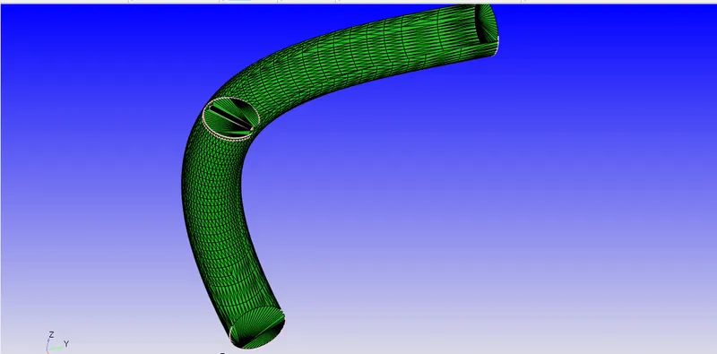
The geometry that was used for the analysis is shown below. An STL file was imported into CONVERGE. It comprised a number of open edges that were cleaned using a Patch command.

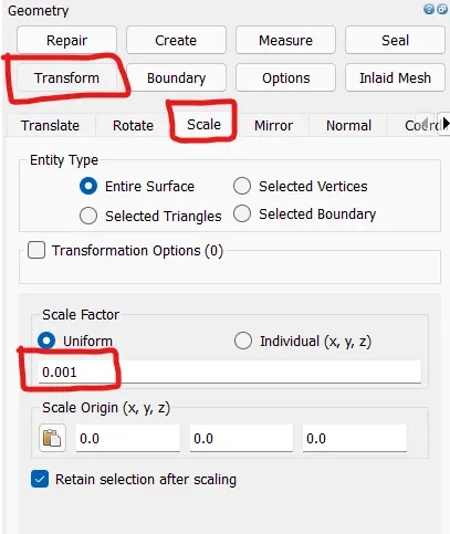
Using the geometry transform option in which scale tool is used to convert the dimension into meters. The scale factor is 0.001 is applied.

After completing the scaling of the geometry, it is required to clean the geometry by closing the flow domain. This is done by finding the boundary with open faces.

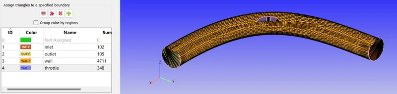
Creation of Boundaries: In the geometry which is created above, boundaries such as inlet, outlet, outer body, and throttle.

The creation of boundaries in the converge studio is the main aspect of meshing geometry. As converge use mesh-free method like cut cell meshing, it requires enclosed geometry for successful operation. The boundary creation is done in the boundary tab of the geometry setup section in which the flag option is used. Four boundaries are created in the setup which is wall, throttle, inlet and outlet. The wall is selected as the elbow's outer space, the throttle is selected as the body inside the elbow. The selection of body inside elbow can be done by hiding elbow after assigning to the boundary which makes only throttle and other faces to be seen. After this, the remaining two faces can be selected as inlet and outlet.

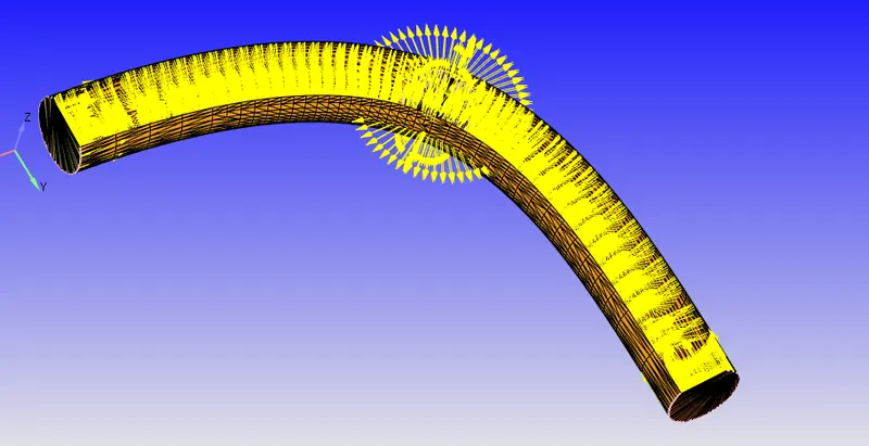
------------------------------------------------------------------------------------------------------------------------Checking Orientation of Normals: Orientation of Normals was checked to ensure all the normals are pointing inwards. This was done using the Normal Toggle.

Finally a Diagnosis check was run to ensure no errors in the geometry.

Materials:- This was set to Air.

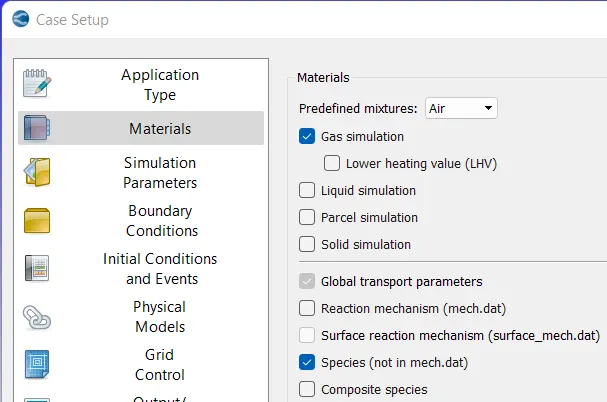
1. i) Gas Simulation: Default properties were retained
2. ii) Global Transport Parameters:- Default properties retained
3. Simulation Parameters

Run Parameters:- Steady state solver was used. Simulation mode was set to Full Hydrodynamic. Gas Flow solver set to Compressible.

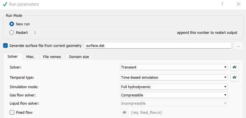
The solver setup is being set up to transient with simulation mode with as full hydrodynamics. The gas flow solver is consider as compressible in nature.

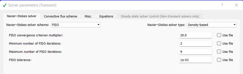
The simulation will be treated as pressure based approach as the velocity of the flow is very low. The Navier-Stoke pressure velocity scheme is consider as PISO as it mostly work for irregular mesh with better convergence.

------------------------------------------------------------------------------------------------------------------------------

Simulation End Time Calculation:

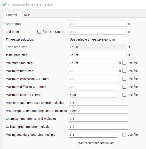
Flow thorugh time is calculated by `v/t = 0.11/80=0.0013` seconds, say 0.002 seconds or 2 milliseconds for fluid to flow once through the pipe. We intend to simulate 5 such movements therefore an end time of 0.01 second is chosen.

The simulation time parameter for the problem is consider as 0.01 seconds. The maximum CFL limit for the problem is again consider as 1 for remove blowout of simulations.

Boundary

- Inlet:- Boundary flow - Inflow

Inlet Pressure- 150000 Pa.

- Outlet- Boundary - Outflow

Outlet Pressure- 100000 Pa.

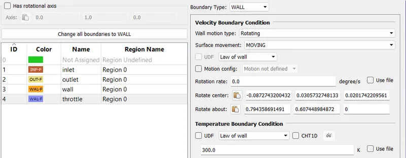
Throttle:- Wall motion was set to Rotating, Surface Movement :- Moving.

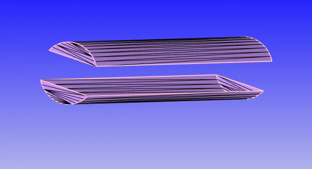
The center and axis of rotation was determined by using the Measure command and Direction Arc Normal. Three points needed to be specified to compute the rod center.

The rod is provided in the CAD.

In this case of transient simulation there is need of rotating the throttle valve because of conditions. To rotate the valve in the prescribe location it require rotation center and the axis around which it is rotating. This co-ordinate can be taken from the converge studio itself using 'Arc Normal' Method. It allows user the measuer the rotating center and rotation axis of the part.

Step 1- Hide the other faces of Throttle. Use Ctrl+H hotkey to hide the surfaces.

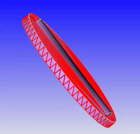
Step 2- Use of Arc Center Method.

In this method user has to select the three vertex location which will provide the required co-cordinates.

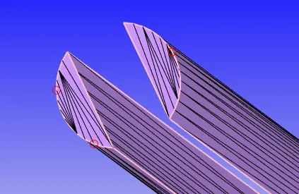
After selecting the three vertex, one has to click apply in the message box it will show the co-ordinates.

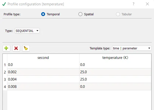
This information has to be feed in the throttle boundary condition with an input file which have the co-ordinate data also the time data with respect to amount of angle by which throttle has to be move.

he motion of throttle valve is given below:

From 0 to 2 milisecond throttle will move by 25 degree

From 2 to 4 milisecond throttle will stay at 25 degree

from 4 to 8 milisecond throttle will come to original position.

It is important to set the input file as .in format or it will not take into account.

4. Initial condition and events

The created geometry was selected as the Volumetric Region.

5. Physical Models:- Default retained.
6. Turbulence Modelling:- RNG-kepsilon turbulence model is used.
7. Grid Control:- A Grid size of 0.002 is entered in dx,dy and dz direction.

Meshing

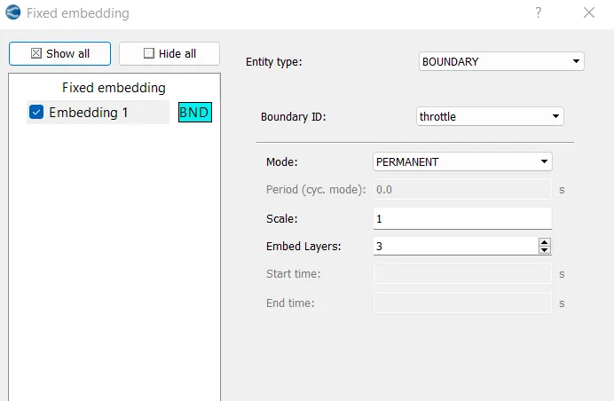
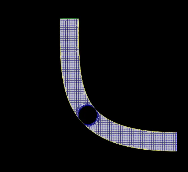
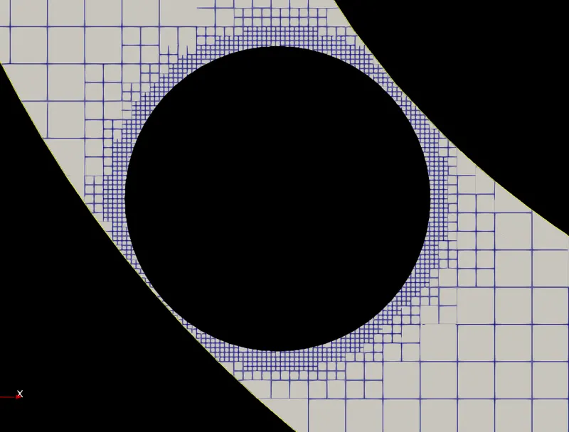
The meshing parameter for the problem is consider as 2mm. The area near the throttle is slender, to capture the flow parameter near the throttle valve it is necessary to create more number of element. This can be done by creating embedding mesh in the region near throttle valve.

------------------------------------------------------------------------------------------------------------------------

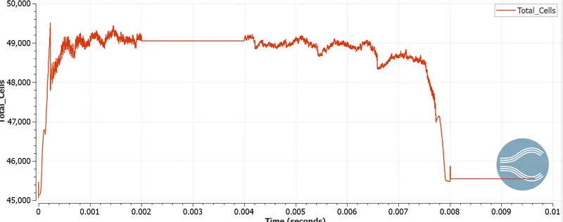
Results:

Mass Flow Rate

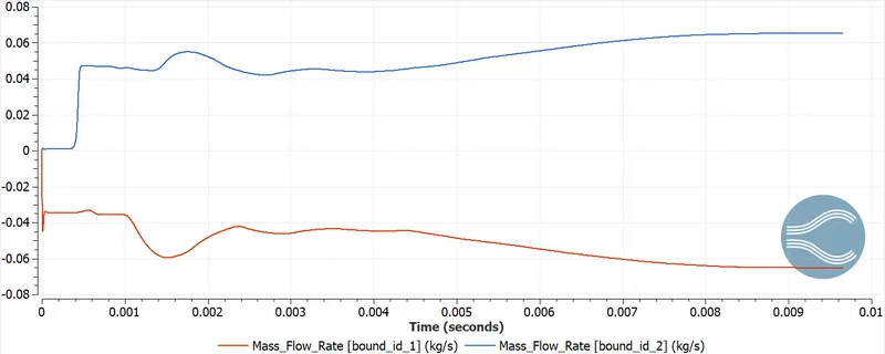
From the above plot we note that the mass flow rates at the inlet and outlet initially vary until 9 milliseconds after which they attain a constant value of 0.06 kg/s for the rest of the simulation

Velocity

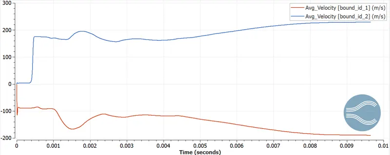
The average velocities too exhibit a similar trend like the Mass flow rate. Until 8 milliseconds,there is a variation after which it attains a constant velocity of around 228 m/s

Pressure

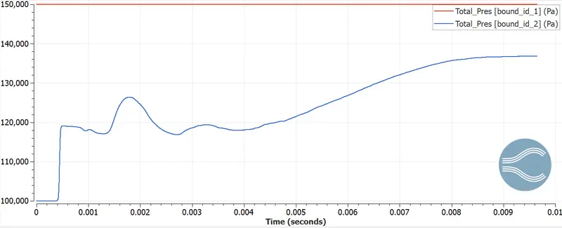
From the above plot it is seen that while the inlet pressure is constant at 150000 Pa, the outlet Pressure reaches a value of little below 136,814 Pa after 8 milliseconds.

-------------------------------------------------------------------------------------------------------------------

Contours

Velocity Contours:- The velocity profile at various time steps is given below.

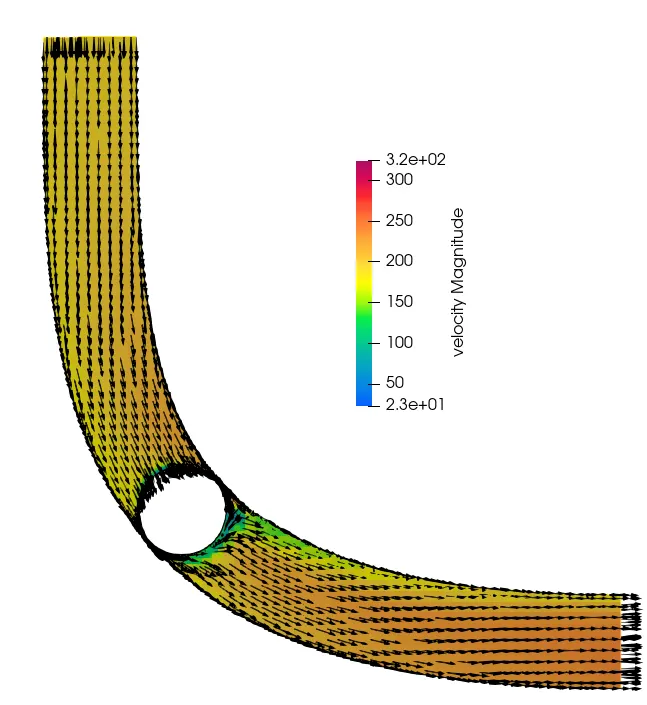
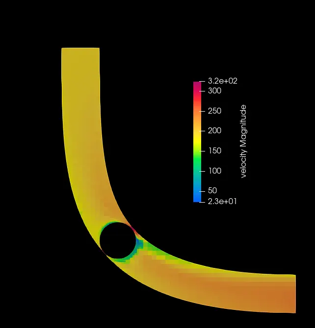
From the contour plots, it is noted that the movement of the throttle valve has a bearing on the outlet velocity. The maximum velocity is achieved when throttle is open, ie it is aligned/ parallel to the flow direction.

Pressure Contours:-

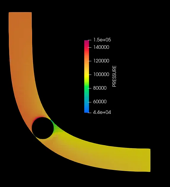
It is noted that movement of throttle valve has an effect on the outlet pressure. When the valve closes it is observed that two distinct pressure zones are created.

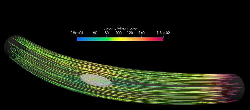
Streamlines:-

------------------------------------------------------------------------------------------------------------------

Conclusion: -

1) From the contour and plot it can be seen that, from the start of deflection of throttle valve, there is an area below the throttle valve have less velocity and it is obstructing the flow very well.

2) From 2.3 milisecond to 4 milisecond the velocity and pressure are nearly stable which can be seen in plot as well as in contours. The velocity lies in the range of 158-161 m/s.

3) The static pressure has been drop in the near vicinity of throttle valve as it has start moving. The total pressure at inlet was around 1.5e5 pascals as stated in the boundary conditions. In the total pressure plot it can be seen that after throttle valve coming to normal position the pressure is increasing and being constant after 8 milisecond to 136,814 pascals.

4) From the transient simulation of throttle valve problem, it can be seen that lowering the area of flow cause the velocity to decrease initially and then sudden increase at the outlet due to sudden expansion of flow.