Week 4.2: Project Transient simulation of flow over a throttle body

Week 4.2: Project Transient simulation of flow over a throttle body

Aim:

• To perform a transient simulation of flow over a throttle body.
• To post process the results and to show the pressure and velocity contours along with the mesh (i.e surface with edges).
• To display the plots for pressure, velocity, mass flow rate and total cell count.
• To calculate the end time for simulation and create an animation in which the throttle movement should be visible.

Throttle body:

• The amount of air that flows into an engine’s combustion chamber is controlled by throttle body which is a part of the air intake system.
• It consists of housing unit that contains a throttle plate that rotates on a shaft.
• Throttle body is located between the air filter and the intake manifold.
• A throttle is a mechanism by which the fluid flow is managed by constriction or obstruction.
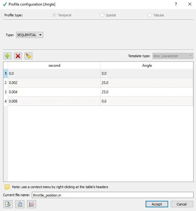
• The mass flow rate is controlled by the angle of the throttle valve. In this project we are going to implement two position parameters of throttle body, in which for the time of 0 to 2 m/s the angle of flipping is 0 to 25 degree and then it remains unchanged till 4 m/s and the throttle reaches it old position at 8 m/s.

Geometry setup:

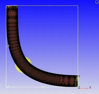
• As the geometry was provided in STL format it is imported in the CONVERGE studio software by using the file--> import --> import STL command.

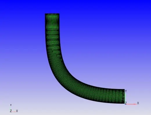
• Diagnosis toolbar is used for geometry check-up.
• The effect of thickness which is responsible for conjugate heat transfer is neglected for this flow over throttle body case.

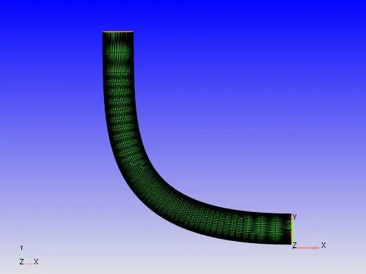
• Then as the geometry as open edges it is closed by using the Geometry dock--> Repair--> Patch--> Free edge loop--> select the open edge and click on apply.

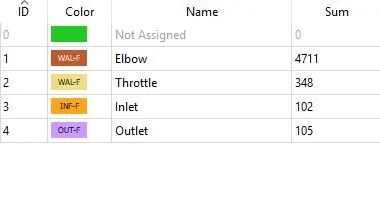
• In the next step the boundaries are flaged with names.

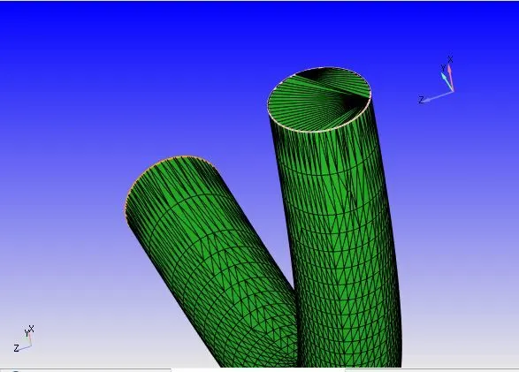
• Then the normal are checked whether they are pointing inside the geometry where the flow passes.

Case Setup:

• The application type is fixed with time based.
• Then click on Materials which is present in the right side of the window that is case setup tree and select the Predefined mixtures as Air.
• Click on the Gas simulation and Global Transport parameter and retain the same values.
• Click on Species and then add O2 and N2.
• Click on Run Parameters and under the solver tab choose the solver as Transient. Set the simulation mode to Full Hydrodynamic and the gas flow solver as compressible.
• Then under "Misc" tab uncheck the use shared memory boxes.
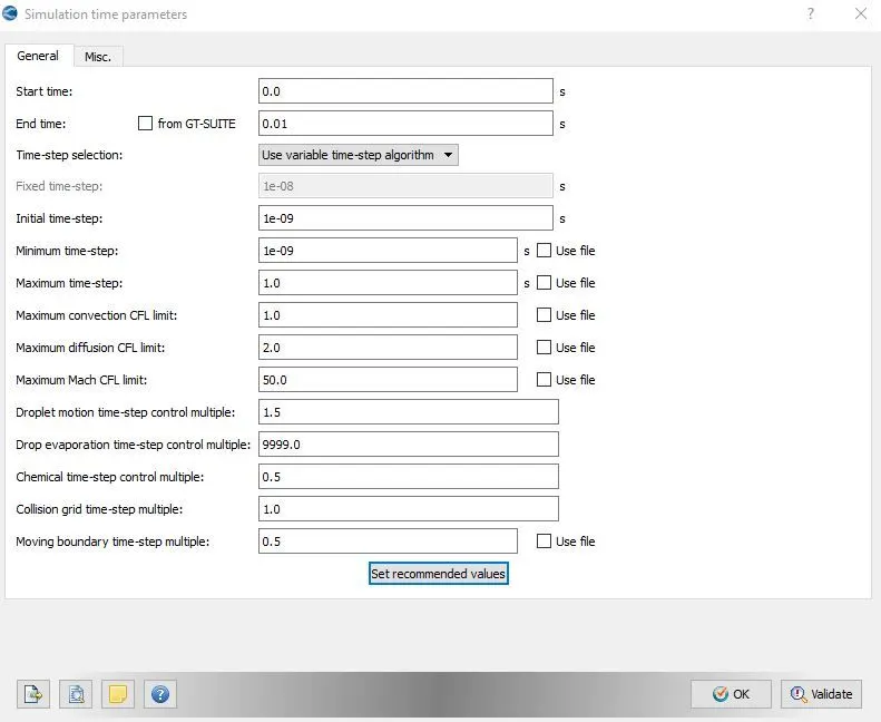
• Under Simulation time parameters enter the end time as 0.01 s.

The end time of the simulation is calculated on the following parameters.

1. Velocity at inlet.

2. Characteristic length of domain.

3. Number of fluid passes through the domain.

The average velocity is 191.43 m/s

The characteristic length of the domain is considered as 0.2m approximately.

So, the time taken to pass a fluid through the elbow = Channel length/Average Velocity.

T=0.2/191.43

T=0.00104 s for one time pass.

Therefore to make a 10 time pass the total end time is 0.01 s approximately

• Then under Solver Parameters select the Navier-Stokes solver type as Pressure Based
• Then coming to Boundary Conditions click on Boundary--> Inlet -->Specify the inlet pressure value as 1.5e5 Pa and select the predefined mixture as Air which contains N2 of 77% and O2 of 23% and then under the Temperature boundary condition choose specified value and allocate the temperature value with 300k.
• Then in Outlet--> Specify the static pressure as 1e5 Pa and select the predefined mixture as Air.
• Then assign the Elbow's boundary condition as Wall.
• Then assign the throttle's boundary condition as Wall. Then assign the wall motion type as Rotating and Surface movement as Moving. Then under the Rotation rate file enter the angle for each time.

• As we are interested in rotating throttle since it was a transient problem, the Rotation center and the Rotation about (axis) will be evaluated using the predefined functions that is available in Converge Studio by using Geometry --> Measure --> Direction --> Arc normal --> Select any three vertices along arc --> apply or Geometry --> Measure --> Direction --> Triangle normal --> select any one triangle --> Apply. A dialog box with the values of rotation center and Rotation about appears in which we could copy the values and enter in the throttle's boundary conditions.

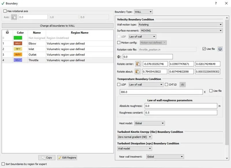
• Then under the Initial conditions and Events --> Regions and Initialization --> add a region and rename it as Volumetric Region User Defined by using the F2 option.
• Then under the boundary conditions assign the region names to the named boundary regions.
• Then under the physical models check the turbulence modelling and set with Reynolds Averaged Navier-Stokes (RANS) and set the turbulence model with RNG K-epsilon.
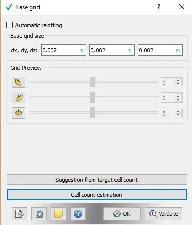
• Then in the Grid Control parameter --> Base Grid --> Enter the size of the grid.

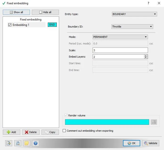
• Then in the Grid control parameter check the "Fixed Embedding" option.
• Enter the values for fixed embedding.

• Then under Output/Post-Processing --> Post Variable Selection --> Add the Mass fraction with O2 and N2
• Then under the Output files --> Writing time intervals --> set the time interval for writing 3D output data files and time interval for writing restarting output.
• Then use CYGWIN to execute the CFD solver.
• Then with the help of Converge CFD the post converting the output files to paraview format is done.
• Paraview is used for Post processing the results.

Results:

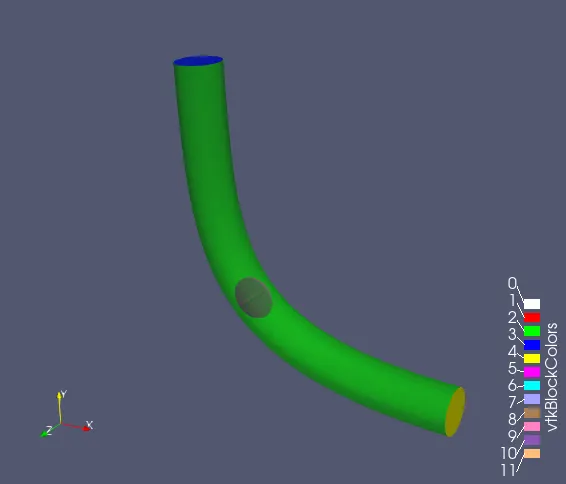
This image represents the throttle body that have been imported in Paraview.

Mesh:

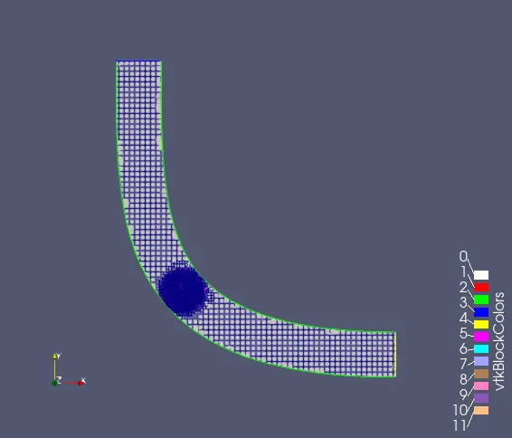
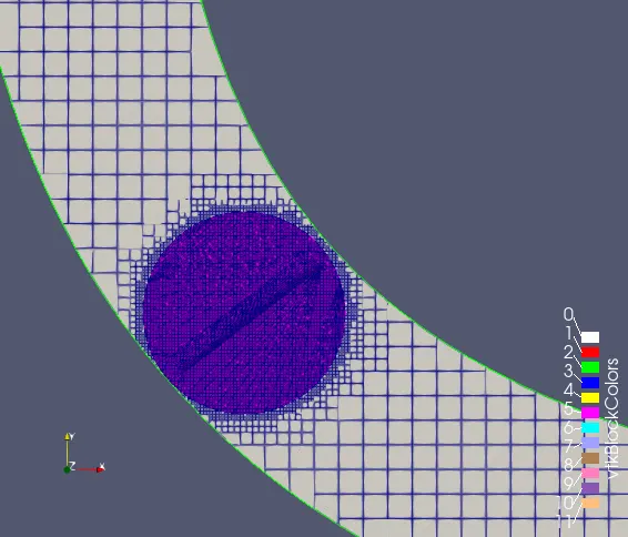
In order to make the mesh really fine near the throttle Fixed embedding is done so that the amount of fluid flow near the throttle leaks through the passages can be accurately calculated. Here we could predict that the mesh around the throttle keeps on changing as throttle moves along the rotation axis.

Mesh Animation:

https://youtu.be/e5X5Ozy3Swg

Velocity Contour:

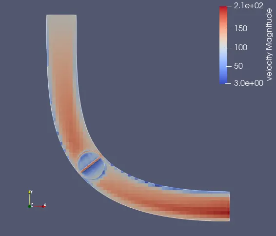
This contour represents the velocity at the initial and final time step where the throttle's angle is at 0 degree change.

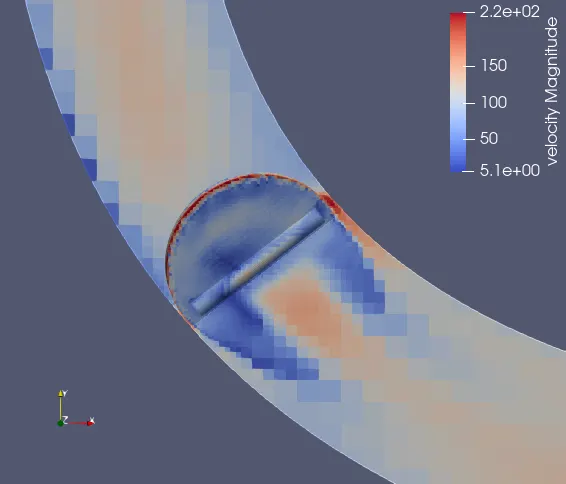
This contour represents the velocity field near the throttle body when it is at an angle of 25 degrees. In this velocity contour we could predict that the velocity drastically increases at the throttle stage and decreases after the throttle. The spread of the wake region decreases when the throttle is positioned at 25 degrees. The stagnation region can be observed at the upstream face of the throttle valve.

Velocity Animation:

https://youtu.be/RaiUglJvjvI

Pressure Contour:

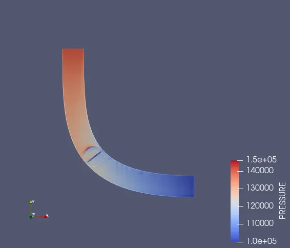
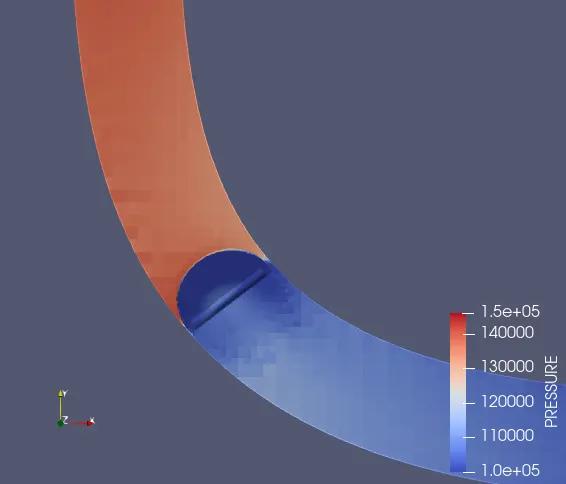
This pressure contour represents the pressure field along the throttle body when it is at it is positioned at 0 degree and 25 degrees respectively. From the second pressure contour we could predict that the pressure drastically increases before the throttle body when it is positioned at 25 degrees. Through this pressure contour we could predict that the pressure increases drastically when the air hits the throttle and it decreases near the elbow walls. The increase in pressure is due to the stagnation and the pressure become normal after the throttle stage.

Pressure Animation:

https://youtu.be/4pGM76yznPQ

https://youtu.be/lO_X_fe6iGg

Mass flow rate plot:

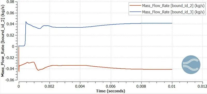
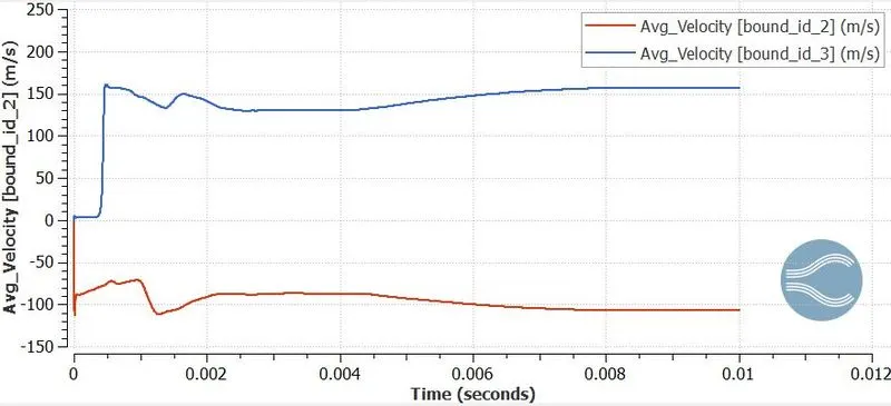
Velocity Plot:

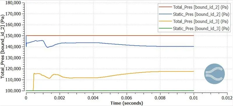
Pressure Plot:

Total Cell Count:

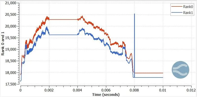
From this plot we could predict that the reason behind this irregular structure of the plot is due to Rotation of Throttle as its position is at 25 degree for particular time the total cell count has a specific value. When the throttle valve starts rotating fixed embedding helps us to provide required amount of grid elements to collect the data throughout the rotation process which results in the change of cell count.

Conclusion:

• The simulation ran successfully showing the transient simulation of the flow behaviour over a rotating throttle. It was observed that the transient simulation takes a longer duration when compared with the steady state simulation. From this transient simulation the procedure for changing the particular boundary's position is well learnt.
• We could observe that when the mesh is finer the contour profile looks detailed at the throttle position as it was created with 2 embedded layer and scaling to 3.
• From the velocity plot we could predict that the inlet velocity profile is inversely proportional to the outlet velocity.
• The total pressure remains constant throughout the flow but the static pressure takes some up and down at the inlet state.
• Restriction of the throttle produces areas of lower velocity and with the closing of throttle the areas of lower velocity increase.
• We could predict the irregular profile in the total cell count. That is because of the change in throttle's position at certain interval of time.
• The cell count increases with the movement in throttle.