Week 4.2: Project Transient simulation of flow over a throttle body
Abstract:
The following report analyses the the transient flow over a throttle body . The velocity and pressure variation with different opening of the throttle body is found out from the simulation. Proper rotation to the throttle body is provided with respect to time .
key words: Throttle body,transient , CFD, Converge studio,
Objective:
- Transient simulation of flow over a throttle body.
- Post-processing the results and explaining the plots and different contours.
- Detailed CFD modelling
The general schema of the following report is that it begins with the theoretical know-how of the throttle body, its uses and applications. The next section that is the CFD modelling contains an exhaustive coverage of all the criterions of the simulation.
Theory:
A throttle body is a butterfly valve located between the air intake filter and the intake manifold. It regulates how much air can go into the engine, based on driver input through the gas pedal. As more air flows into the engine, it injects more fuel, thus allowing for more power. Throttle bodies today are mostly electronically controlled, where this throttle body is mechanical. It includes input for TPS and MAP sensors, as well as routing for the IAC valve, and a idle adjustment screw.
A throttle is the mechanism by which fluid flow is managed by constriction or obstruction.An engine's power can be increased or decreased by the restriction of inlet gases (by the use of a throttle), but usually decreased. The term throttle has come to refer, informally, to any mechanism by which the power or speed of an engine is regulated, such as a car's accelerator pedal. What is often termed a throttle (in an aviation context) is also called a thrust lever particularly for jet engine powered aircraft. For a steam locomotive the valve which controls the steam is known as the regulator
CFD Modelling:
The flow chart or the procedure is
- Creating Geometry / Importing Geometry
- Debugging the geometry if any
- Boundary flagging or creating boundaries
- Case set up
- running the simulation and post processing.
1) Geometry :
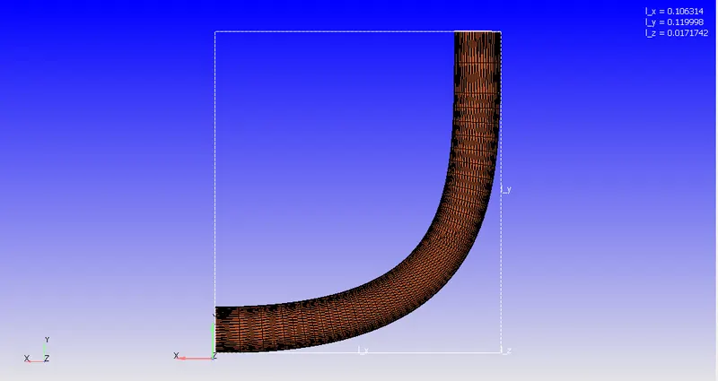
The cad file (read stl) is imported into Converge studio. The unique feature of Converge studio is that , it discretizes the geometry in triangles as building blocks. The diagnosis is run, and the errors shown are open edges. The open edges are removed by using the patch tool.
The boundary flagging is done to create boundaries .
- Elbow walls- This constitutes the wall of the elbow.
- Inlet- The region through which the fluid enters
- Outlet- the region through which the fluid exits
- Throttle body- The throttle body is present inside the geometry. It is seen that the throttle body type is surface .
2) Case set up:
- Application type:
The application type is time based . The time is measured in seconds.
- Materials :
The predefined mixture is air. Gas simulation is checked. The species box is checked.
The redlich-Kwon equation of state is selected.
The turbulent prandtl number is 0.9 and the turbulent scmidt number is 0.78.
The species are O2 and N2.
- Simulation run parameters:
Transient state simulation is done for compressible flow in a full hydrodynamic mode. No hydrodynamic mode is selected to check the meshing and the set up. In that case the Navier stokes equation are not solved, only the mesh generation is checked.
- Simulation time parameters:
The start time and the end time is in seconds as the simulation is transient. The end time is calculated by the following procedure:
The length of the elbow is 0.2 meters (maximum). the average velocity is roughly 80 m/s. So the time in seconds is 0.2/80= 2.5 *10^-3 = 2.5 miliseconds. This means the One tome step is 2.5 miliseconds. To calculate for four time steps, the end time is 2.5*10^-3*4=0.1 seconds.
Initial time step and the minimum time step is 1e-9 seconds.
The maximum time step is 1 seconds.
The maximum convecxtion CFL limit is 1 and the maximum diffusion CFL limit is 2.
- Solver parameters:
The Navier stokes solver scheme selected is PISO. The two availble solver schemes are PISO and SIMPLE.
Density based solver is used.
- Boundary conditions:
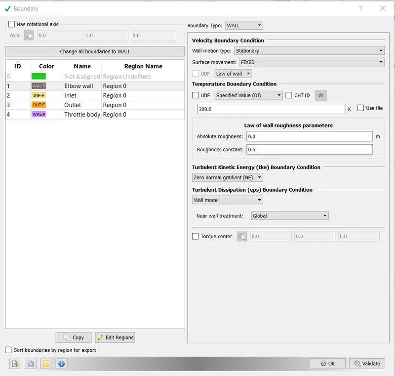
1) Elbow wall:
The boundary type is Wall. The wall motion is stationary and the surface movement is fixed and follows the Law of the wall. Law of wall condition is generally assigned to flyid regions.
The temperature boundary condition is specified at 300 K.
2)Inlet:
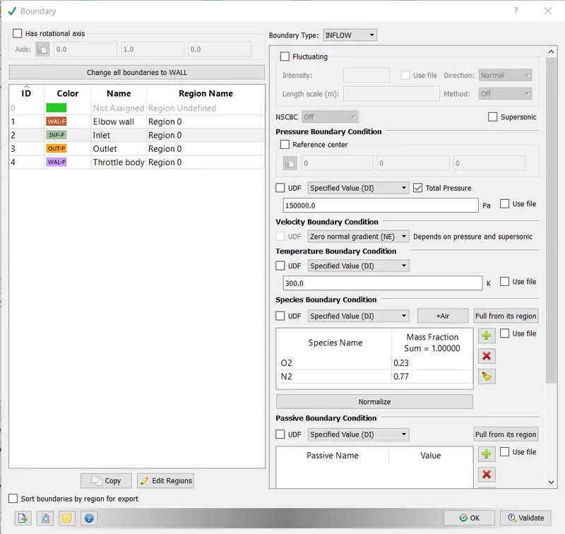
The Boundary type is Inflow.
The pressure is specified as 150000 pas.
The velocity boundary conditions follows a Zero normal gradient and the Temperature boundary condirtion is specified as 300K.
The species at the inlet is Air.
3) Outlet:
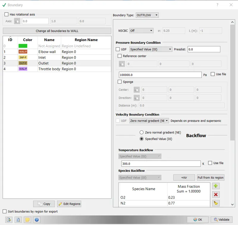
The Boundary type is outflow. The pressure at the outlet is specified as 100000 pas. the velocity boundary conditions follows The zero normal gradient and the backflow species is Air.
4) Throttle Body:
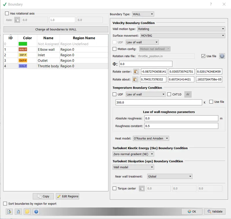
Boundary type is wall. The wall motion type is rotating and the surface movement is moving and follows the law of the wall.
Rotation rate file : The rotation rate file is specified such that , at the 0 seconds the throttle is closed. at the 2 miliseconds the throttle rotates about 25 degress. t 4 miliseconds the throttle rotates about 25 degress. And after that at 8 miliseonds the throttle comes to the original position. To do that , a file is used named throttle_position.in.
Rotation center:
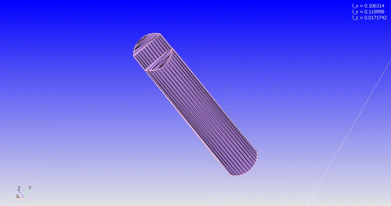
In the above image , the cylinder of the throttle is shown . the top of that cylimder xan be imagined as a section of a circle. Rotation center is the center of that circle. to find that, we go to measure then direction then arc normal. Three points are chosen . Two in one half, one in anpther, When clicked apply, the rotation center and the rotation about is found out.
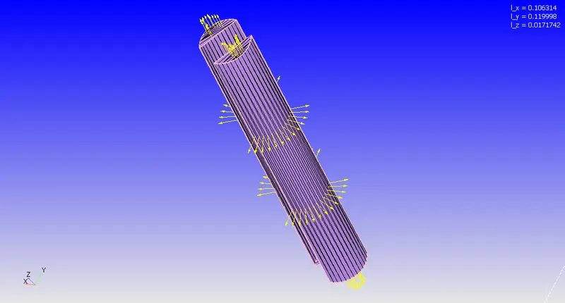
Rotaion about is thge orientation of the normals. This can be found out also using the triangle method.
Temperture boundary conditions follows the law of the wall.
- Regions and initializations:
The region id is region0. the species air is pulled in . temperature and pressure are specified as 300K and 101325 pas.
Under the physical modelling , only turbulence modelling is selected.
- Turbulence modelling:
RANS and the turbulence model selected is RNG K-epsilon. Other parameters are selected as default selection by converge studio.
- Base grid:
the base grid selected is dx=0.002 meters , dy=0.002 meters and dz=0.002 meters.
The cell count estimated without embeddment is 5904 cells.
Fixed embedding':
Entity type is boundary and the boundary id is throttle body.
The scale is 3 and the number of layers selected is 2.
The Post variable selection is left as default selection by converge studio.
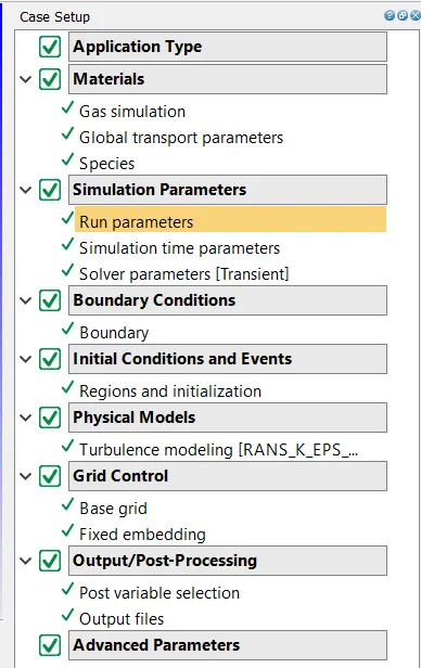
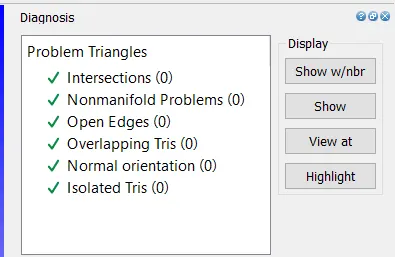
The case set up dock and the diagnosis ran :
3) Simulation
The input files are stored in a folder. The vommand prompt is openned. After copying the mpi executab;le and the converge run exectuable, the command followed after getting inside the directory is
'moiexec.exe -n 4 converge.exe restricted'
The 4 signifis the number of processir used .
4) Post-processing and the results:
The line plots obtained in the converge studio after the simulation ended are:
- Cell counts:
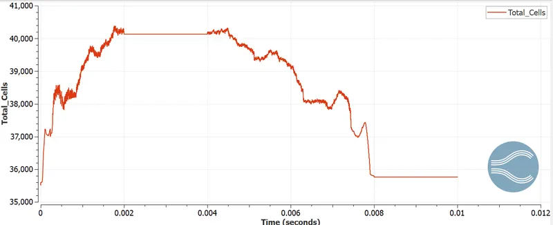
The total cell count nearly rose to 36000.
- Average velocity at inlet and outlet:
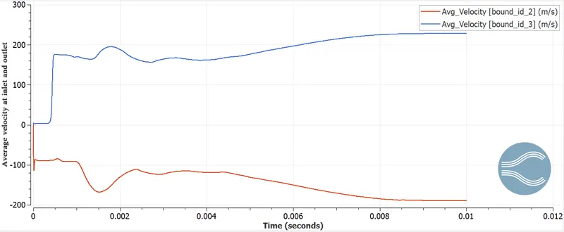
The average velocity at the inlet and outlet is plotted simultaneously in a same plot.
- static pressure, total pressure at inlet and outlet:
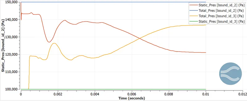
The static pressire and total pressure at inlet and outlet is plotted along the inlet and outlet.
- Mass flow rate at inlet and outlet:
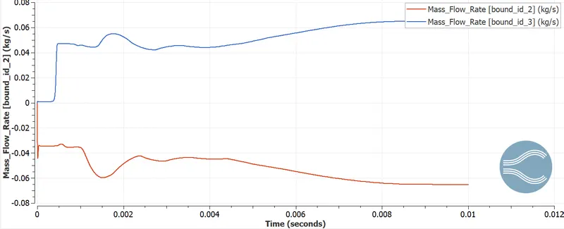
Mass flow rates at the inlet and outlet is plotted.
post processed contours in paraview:
- Grid generation:
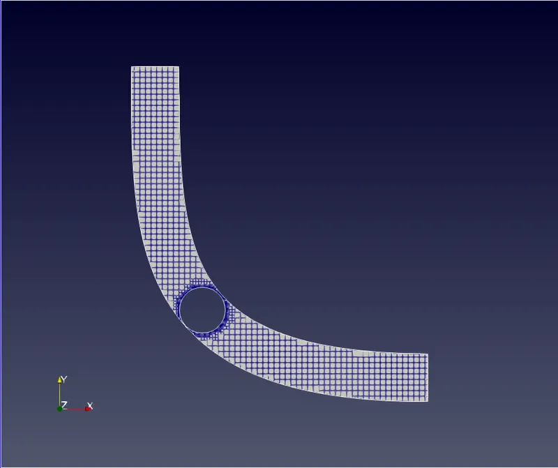
The grid generation is shown . The fixed embedding can be visualized along the throttle boundary.
- Velocity contour:
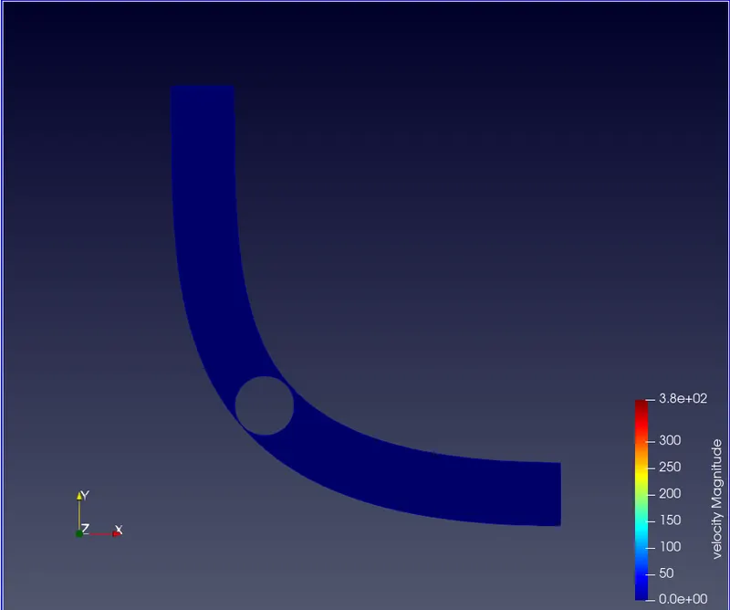
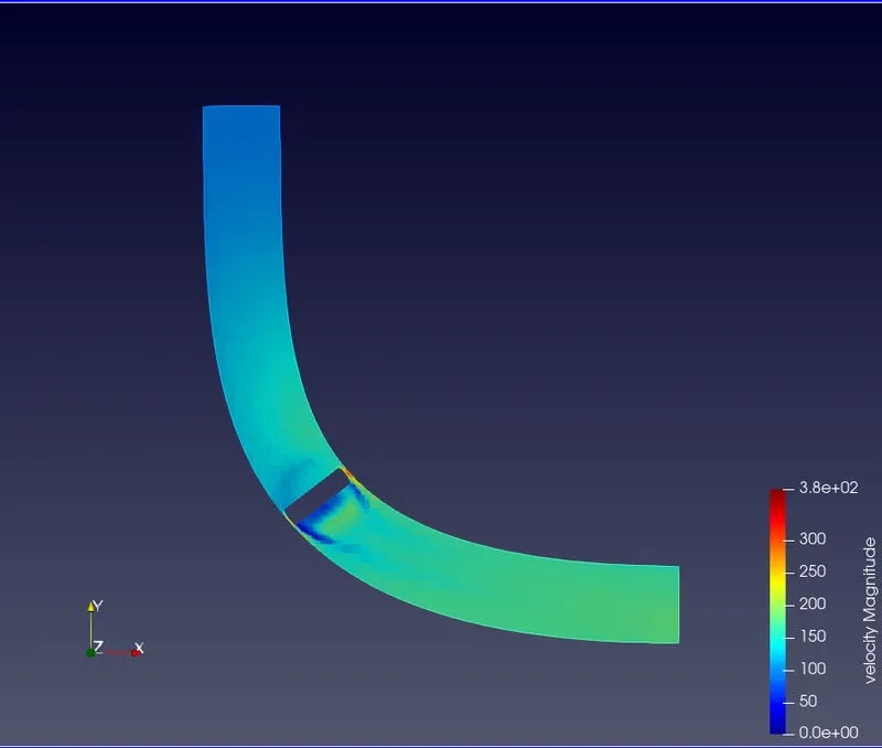
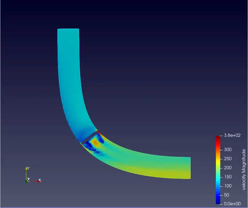
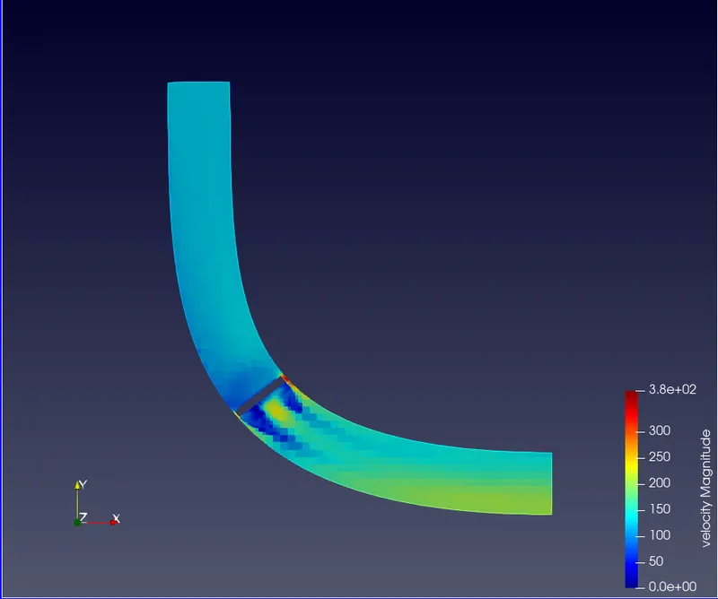
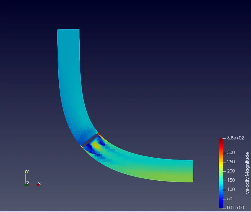
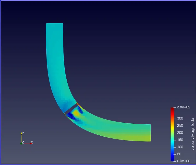
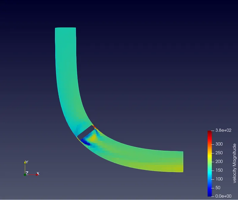
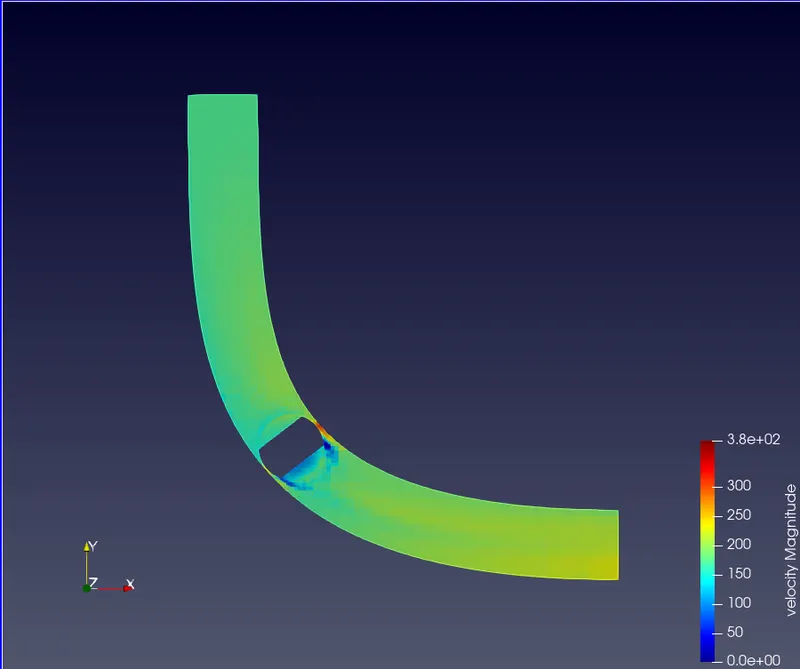
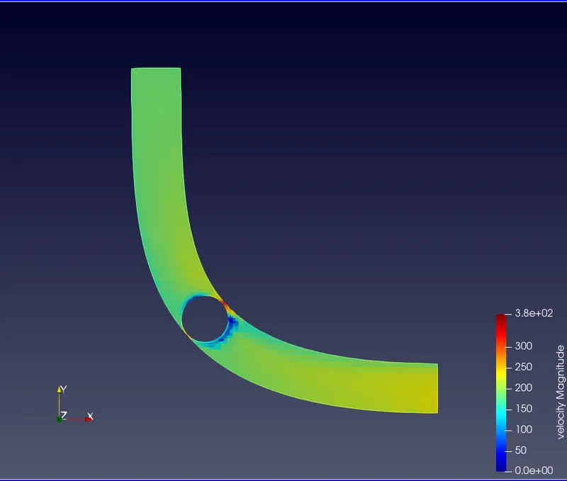
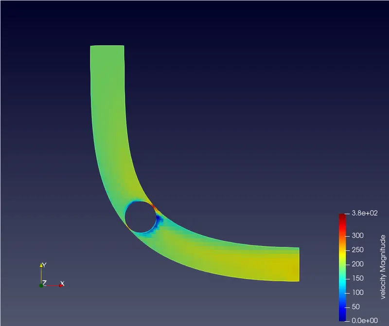
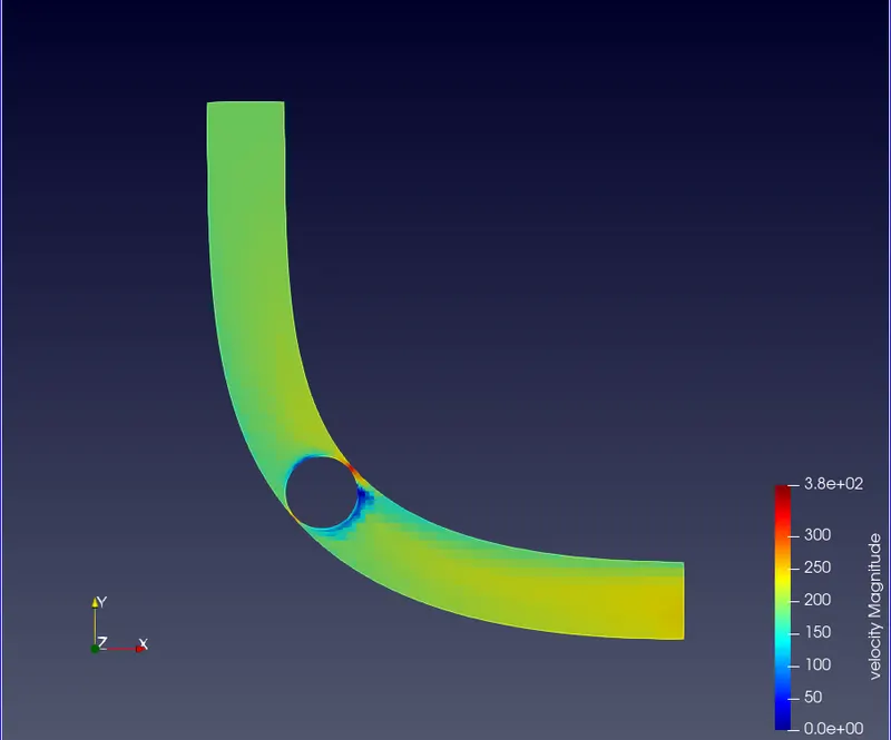
The above contours shows the change in velocity through out the cutplane during all the time steps. It can be noticed that the throttle body moves by 25 degrees and then gets fully open. Subsequent velocity variation can be noticed.
- Pressure contour:
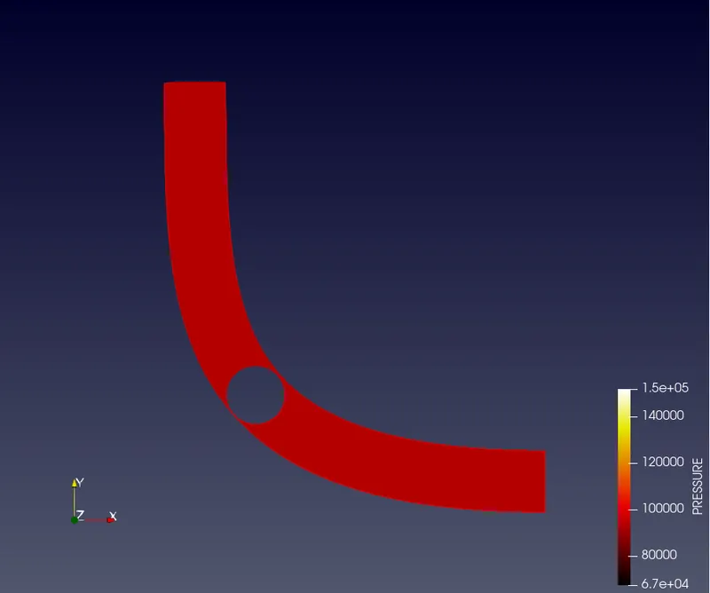
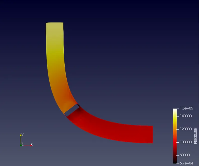
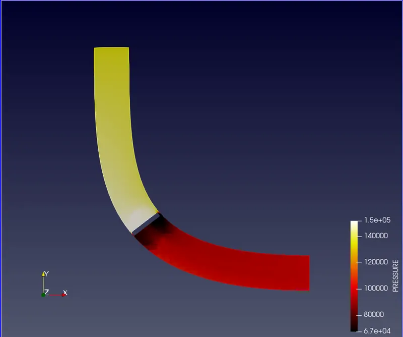
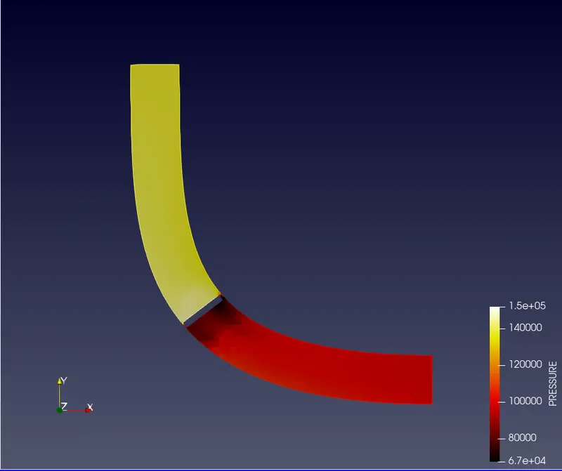
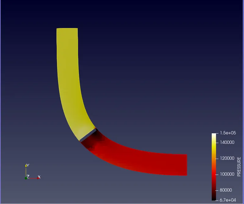
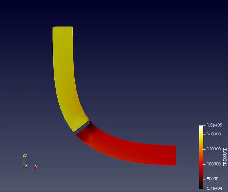
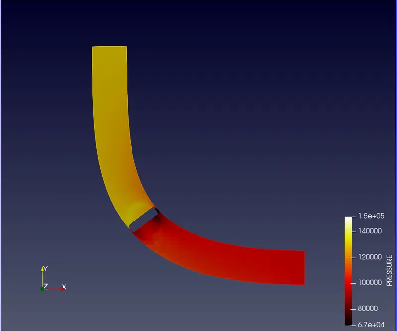
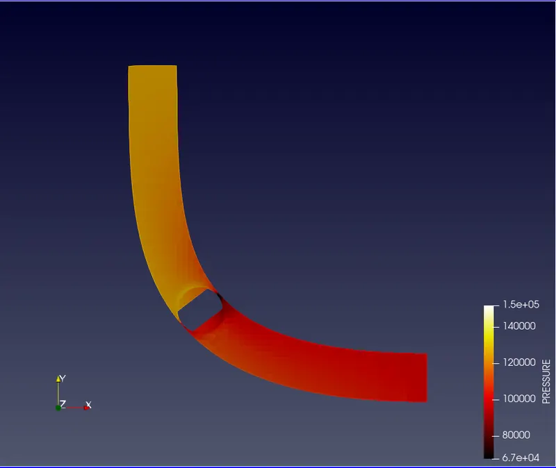
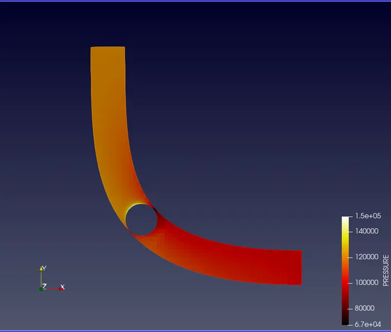
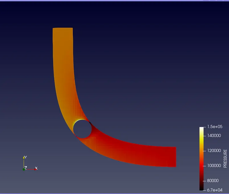
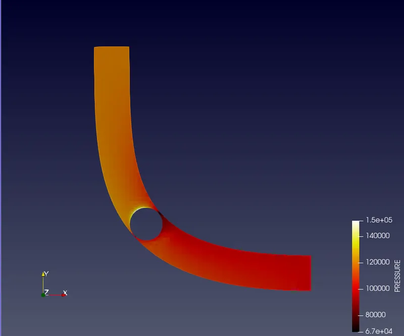
The pressure variation at different throttle body movemnet is shown above.
- Animation:
1) Velocity:
The link to the youtube video is: https://youtu.be/PxnqRC9rB28
2) Pressure :
The link to the youtube video is : https://youtu.be/8eoaIKGEN70
3) Simulation of streamlines with the throttle body movement visible:
Number of streamlines is 120 . The throttle body movement is visible. The throttle body is coloured with pressure.
4) Pressure variation in the throttle body:
Conclusion:
- The transient simulation of flow over throttle body is studied.
- The Calculation of end time in simulation time parameters is shown.
- The rotation of the throttle body about the rotation center is described in details.
- The velocity and pressure variation along the time steps with the different opening of the throttle body is visualized.